Downloaded 10 times
![Transforming Differential Equation
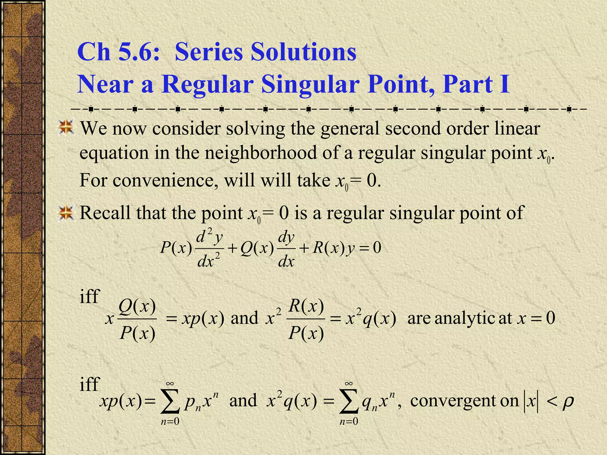
Our differential equation has the form
Dividing by P(x) and multiplying by x2
, we obtain
Substituting in the power series representations of p and q,
we obtain
0)()()( =+′+′′ yxRyxQyxP
∑∑
∞
=
∞
=
==
0
2
0
,)(,)(
n
n
n
n
n
n xqxqxxpxxp
[ ] [ ] 0)()( 22
=+′+′′ yxqxyxxpxyx
( ) ( ) 02
210
2
210
2
=++++′++++′′ yxqxqqyxpxppxyx ](https://image.slidesharecdn.com/ch056-150731094716-lva1-app6892/85/Ch05-6-2-320.jpg)
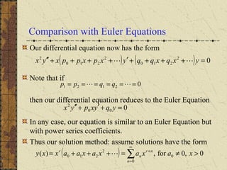
![Example 1: Euler Equation (2 of 13)
Now xp(x) = -1/2 and x2
q(x) = (1 + x )/2, and thus for
it follows that
Thus the corresponding Euler Equation is
As in Section 5.5, we obtain
We will refer to this result later.
0,2/1,2/1,2/1 3221100 ========−= qqppqqp
∑∑
∞
=
∞
=
==
0
2
0
,)(,)(
n
n
n
n
n
n xqxqxxpxxp
020 2
00
2
=+′−′′⇔=+′+′′ yyxyxyqyxpyx
[ ] ( )( ) 2/1,1011201)1(2 ==⇔=−−⇔=+−− rrrrrrrxr
( ) 012 2
=++′−′′ yxyxyx](https://image.slidesharecdn.com/ch056-150731094716-lva1-app6892/85/Ch05-6-5-320.jpg)
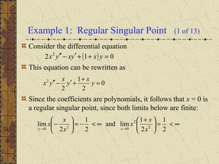
![Example 1: Combining Series (4 of 13)
Our equation
can next be written as
It follows that
and
( )( ) ( ) 012
1
1
000
=+++−−++ ∑∑∑∑
∞
=
+
−
∞
=
+
∞
=
+
∞
=
+
n
nr
n
n
nr
n
n
nr
n
n
nr
n xaxaxnraxnrnra
[ ] ( )( )[ ]{ } 01)(121)1(2
1
10 =+++−−++++−− ∑
∞
=
+
−
n
nr
nn
r
xanrnrnraxrrra
[ ] 01)1(20 =+−− rrra
( )( )[ ] ,2,1,01)(12 1 ==+++−−++ − nanrnrnra nn](https://image.slidesharecdn.com/ch056-150731094716-lva1-app6892/85/Ch05-6-7-320.jpg)
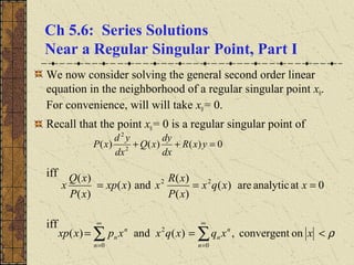
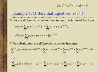
![Example 1: Indicial Equation (5 of 13)
From the previous slide, we have
The equation
is called the indicial equation, and was obtained earlier when
we examined the corresponding Euler Equation.
The roots r1= 1, r2 = ½, of the indicial equation are called the
exponents of the singularity, for regular singular point x = 0.
The exponents of the singularity determine the qualitative
behavior of solution in neighborhood of regular singular point.
[ ] 0)1)(12(13201)1(2 2
0
0
0
=−−=+−⇔=+−−
≠
rrrrrrra
a
[ ] ( )( )[ ]{ } 01)(121)1(2
1
10 =+++−−++++−− ∑
∞
=
+
−
n
nr
nn
r
xanrnrnraxrrra](https://image.slidesharecdn.com/ch056-150731094716-lva1-app6892/85/Ch05-6-8-320.jpg)
![Example 1: Recursion Relation (6 of 13)
Recall that
We now work with the coefficient on xr+n
:
It follows that
[ ] ( )( )[ ]{ } 01)(121)1(2
1
10 =+++−−++++−− ∑
∞
=
+
−
n
nr
nn
r
xanrnrnraxrrra
( )( )[ ] 01)(12 1 =+++−−++ −nn anrnrnra
( )( )
( )
( )[ ] ( )[ ]
1,
112
1)(32
1)(12
1
2
1
1
≥
−+−+
−=
++−+
−=
++−−++
−=
−
−
−
n
nrnr
a
nrnr
a
nrnrnr
a
a
n
n
n
n](https://image.slidesharecdn.com/ch056-150731094716-lva1-app6892/85/Ch05-6-9-320.jpg)
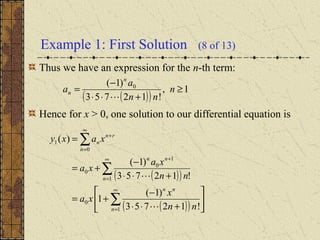
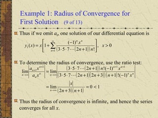
![Example 1: First Root (7 of 13)
We have
Starting with r1= 1, this recursion becomes
Thus
( )[ ] ( )[ ]
2/1and1,1for,
112
11
1
==≥
−+−+
−= −
rrn
nrnr
a
a n
n
( )[ ] ( )[ ] ( )
1,
1211112
11
≥
+
−=
−+−+
−= −−
n
nn
a
nn
a
a nn
n
( )( )215325
13
01
2
0
1
⋅⋅
=
⋅
−=
⋅
−=
aa
a
a
a
( )( )
( )( )
1,
!12753
)1(
etc,
32175337
0
02
3
≥
+⋅⋅
−
=
⋅⋅⋅⋅
−=
⋅
−=
n
nn
a
a
aa
a
n
n
](https://image.slidesharecdn.com/ch056-150731094716-lva1-app6892/85/Ch05-6-10-320.jpg)
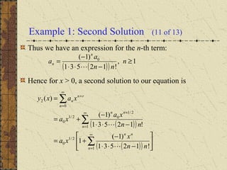
![Example 1: Second Root (10 of 13)
Recall that
When r1= 1/2, this recursion becomes
Thus
( )[ ] ( )[ ]
2/1and1,1for,
112
11
1
==≥
−+−+
−= −
rrn
nrnr
a
a n
n
( )[ ] ( )[ ] ( ) ( )
1,
122/1212/112/12
111
≥
−
−=
−
−=
−+−+
−= −−−
n
nn
a
nn
a
nn
a
a nnn
n
( )( )312132
11
01
2
0
1
⋅⋅
=
⋅
−=
⋅
−=
aa
a
a
a
( )( )
( ) ( )( )
1,
!12531
)1(
etc,
53132153
0
02
3
≥
−⋅⋅
−
=
⋅⋅⋅⋅
−=
⋅
−=
n
nn
a
a
aa
a
n
n
](https://image.slidesharecdn.com/ch056-150731094716-lva1-app6892/85/Ch05-6-13-320.jpg)
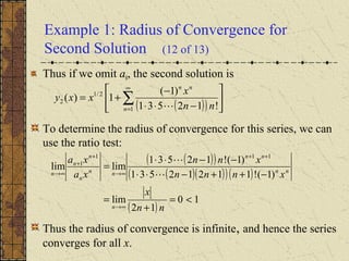
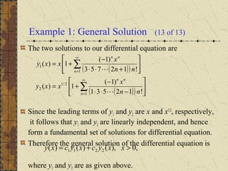
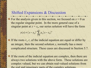

This document discusses solving second-order linear differential equations near a regular singular point, which is done by assuming power series solutions and obtaining recursion relations between the coefficients. Specifically, it provides an example of solving the differential equation ( ) 012 2=++′−′′ yxyxyx near the regular singular point x=0. Two linearly independent solutions are obtained in the forms of ( )( )∑∞=1!12753)1( nnnxaxy and ( )( )∑∞=12/1!12531)1( nnnxaxy , yielding the general solution ( )0),()()( 2211 >+= xxycxycxy .