3c3 nonhomgen lineqns-stuhuhuhuhuhh

Nonhomogeneous Linear Equations
In this section we learn how to solve second-order nonhomogeneous linear differential equa-
tions with constant coefficients, that is, equations of the form
where , , and are constants and is a continuous function. The related homogeneous
equation
is called the complementary equation and plays an important role in the solution of the
original nonhomogeneous equation (1).
Theorem The general solution of the nonhomogeneous differential equation (1)
can be written as
where is a particular solution of Equation 1 and is the general solution of the
complementary Equation 2.
Proof All we have to do is verify that if is any solution of Equation 1, then is a
solution of the complementary Equation 2. Indeed
We know from Additional Topics: Second-Order Linear Differential Equations how to
solve the complementary equation. (Recall that the solution is , where
and are linearly independent solutions of Equation 2.) Therefore, Theorem 3 says that
we know the general solution of the nonhomogeneous equation as soon as we know a par-
ticular solution . There are two methods for finding a particular solution: The method of
undetermined coefficients is straightforward but works only for a restricted class of func-
tions . The method of variation of parameters works for every function but i0s usually
more difficult to apply in practice.
The Method of Undetermined Coefficients
We first illustrate the method of undetermined coefficients for the equation
where ) is a polynomial. It is reasonable to guess that there is a particular solution
that is a polynomial of the same degree as because if is a polynomial, then
is also a polynomial. We therefore substitute a polynomial (of the
same degree as ) into the differential equation and determine the coefficients.
EXAMPLE 1 Solve the equation .
SOLUTION The auxiliary equation of is
r2
ϩ r Ϫ 2 ෇ ͑r Ϫ 1͒͑r ϩ 2͒ ෇ 0
yЉ ϩ yЈ Ϫ 2y ෇ 0
yЉ ϩ yЈ Ϫ 2y ෇ x2
G
yp͑x͒ ෇ayЉ ϩ byЈ ϩ cy
yGyp
G͑x
ayЉ ϩ byЈ ϩ cy ෇ G͑x͒
GG
yp
y2
y1yc ෇ c1y1 ϩ c2y2
෇ t͑x͒ Ϫ t͑x͒ ෇ 0
෇ ͑ayЉ ϩ byЈ ϩ cy͒ Ϫ ͑aypЉ ϩ bypЈ ϩ cyp ͒
a͑y Ϫ yp ͒Љ ϩ b͑y Ϫ yp ͒Ј ϩ c͑y Ϫ yp ͒ ෇ ayЉ Ϫ aypЉ ϩ byЈ Ϫ bypЈ ϩ cy Ϫ cyp
y Ϫ ypy
ycyp
y͑x͒ ෇ yp͑x͒ ϩ yc͑x͒
3
ayЉ ϩ byЈ ϩ cy ෇ 02
Gcba
ayЉ ϩ byЈ ϩ cy ෇ G͑x͒1
1

with roots , . So the solution of the complementary equation is
Since is a polynomial of degree 2, we seek a particular solution of the form
Then and so, substituting into the given differential equation, we
have
or
Polynomials are equal when their coefﬁcients are equal. Thus
The solution of this system of equations is
A particular solution is therefore
and, by Theorem 3, the general solution is
If (the right side of Equation 1) is of the form , where and are constants,
then we take as a trial solution a function of the same form, , because the
derivatives of are constant multiples of .
EXAMPLE 2 Solve .
SOLUTION The auxiliary equation is with roots , so the solution of the
complementary equation is
For a particular solution we try . Then and . Substi-
tuting into the differential equation, we have
so and . Thus, a particular solution is
and the general solution is
If is either or , then, because of the rules for differentiating the
sine and cosine functions, we take as a trial particular solution a function of the form
yp͑x͒ ෇ A cos kx ϩ B sin kx
C sin kxC cos kxG͑x͒
y͑x͒ ෇ c1 cos 2x ϩ c2 sin 2x ϩ
1
13 e3x
yp͑x͒ ෇
1
13 e3x
A ෇
1
1313Ae3x
෇ e3x
9Ae3x
ϩ 4͑Ae3x
͒ ෇ e3x
ypЉ ෇ 9Ae3x
ypЈ ෇ 3Ae3x
yp͑x͒ ෇ Ae3x
yc͑x͒ ෇ c1 cos 2x ϩ c2 sin 2x
Ϯ2ir2
ϩ 4 ෇ 0
yЉ ϩ 4y ෇ e3x
ek x
ek x
yp͑x͒ ෇ Aek x
kCCek x
G͑x͒
y ෇ yc ϩ yp ෇ c1ex
ϩ c2 eϪ2x
Ϫ
1
2 x2
Ϫ
1
2 x Ϫ
3
4
yp͑x͒ ෇ Ϫ
1
2 x2
Ϫ
1
2 x Ϫ
3
4
C ෇ Ϫ
3
4B ෇ Ϫ
1
2A ෇ Ϫ
1
2
2A ϩ B Ϫ 2C ෇ 02A Ϫ 2B ෇ 0Ϫ2A ෇ 1
Ϫ2Ax2
ϩ ͑2A Ϫ 2B͒x ϩ ͑2A ϩ B Ϫ 2C͒ ෇ x2
͑2A͒ ϩ ͑2Ax ϩ B͒ Ϫ 2͑Ax2
ϩ Bx ϩ C͒ ෇ x2
ypЉ ෇ 2AypЈ ෇ 2Ax ϩ B
yp͑x͒ ෇ Ax2
ϩ Bx ϩ C
G͑x͒ ෇ x2
yc ෇ c1ex
ϩ c2 eϪ2x
Ϫ2r ෇ 1
2 ■ NONHOMOGENEOUS LINEAR EQUATIONS
■ ■ Figure 1 shows four solutions of the differen-
tial equation in Example 1 in terms of the particu-
lar solution and the functions
and .t͑x͒ ෇ eϪ2x
f ͑x͒ ෇ exyp
■ ■ Figure 2 shows solutions of the differential
equation in Example 2 in terms of and the
functions and .
Notice that all solutions approach as
and all solutions resemble sine functions when
is negative.x
x l ϱϱ
t͑x͒ ෇ sin 2xf ͑x͒ ෇ cos 2x
yp
FIGURE 1
8
_5
_3 3
yp
yp+3g
yp+2f
yp+2f+3g
FIGURE 2
4
_2
_4 2
yp
yp+g
yp+f
yp+f+g

NONHOMOGENEOUS LINEAR EQUATIONS ■ 3
EXAMPLE 3 Solve .
SOLUTION We try a particular solution
Then
so substitution in the differential equation gives
or
This is true if
The solution of this system is
so a particular solution is
In Example 1 we determined that the solution of the complementary equation is
. Thus, the general solution of the given equation is
If is a product of functions of the preceding types, then we take the trial solu-
tion to be a product of functions of the same type. For instance, in solving the differential
equation
we would try
If is a sum of functions of these types, we use the easily veriﬁed principle of super-
position, which says that if and are solutions of
respectively, then is a solution of
EXAMPLE 4 Solve .
SOLUTION The auxiliary equation is with roots , so the solution of the com-
plementary equation is . For the equation we try
Then , , so substitution in the equation
gives
or ͑Ϫ3Ax ϩ 2A Ϫ 3B͒ex
෇ xex
͑Ax ϩ 2A ϩ B͒ex
Ϫ 4͑Ax ϩ B͒ex
෇ xex
yp1
Љ ෇ ͑Ax ϩ 2A ϩ B͒ex
yp1
Ј ෇ ͑Ax ϩ A ϩ B͒ex
yp1
͑x͒ ෇ ͑Ax ϩ B͒ex
yЉ Ϫ 4y ෇ xex
yc͑x͒ ෇ c1e2x
ϩ c2 eϪ2x
Ϯ2r2
Ϫ 4 ෇ 0
yЉ Ϫ 4y ෇ xex
ϩ cos 2x
ayЉ ϩ byЈ ϩ cy ෇ G1͑x͒ ϩ G2͑x͒
yp1
ϩ yp2
ayЉ ϩ byЈ ϩ cy ෇ G2͑x͒ayЉ ϩ byЈ ϩ cy ෇ G1͑x͒
yp2
yp1
G͑x͒
yp͑x͒ ෇ ͑Ax ϩ B͒ cos 3x ϩ ͑Cx ϩ D͒ sin 3x
yЉ ϩ 2yЈ ϩ 4y ෇ x cos 3x
G͑x͒
y͑x͒ ෇ c1ex
ϩ c2 eϪ2x
Ϫ
1
10 ͑cos x ϩ 3 sin x͒
yc ෇ c1ex
ϩ c2eϪ2x
yp͑x͒ ෇ Ϫ
1
10 cos x Ϫ
3
10 sin x
B ෇ Ϫ
3
10A ෇ Ϫ
1
10
ϪA Ϫ 3B ෇ 1andϪ3A ϩ B ෇ 0
͑Ϫ3A ϩ B͒ cos x ϩ ͑ϪA Ϫ 3B͒ sin x ෇ sin x
͑ϪA cos x Ϫ B sin x͒ ϩ ͑ϪA sin x ϩ B cos x͒ Ϫ 2͑A cos x ϩ B sin x͒ ෇ sin x
ypЉ ෇ ϪA cos x Ϫ B sin xypЈ ෇ ϪA sin x ϩ B cos x
yp͑x͒ ෇ A cos x ϩ B sin x
yЉ ϩ yЈ Ϫ 2y ෇ sin x

Thus, and , so , , and
For the equation , we try
Substitution gives
or
Therefore, , , and
By the superposition principle, the general solution is
Finally we note that the recommended trial solution sometimes turns out to be a solu-
tion of the complementary equation and therefore can’t be a solution of the nonhomoge-
neous equation. In such cases we multiply the recommended trial solution by (or by
if necessary) so that no term in is a solution of the complementary equation.
EXAMPLE 5 Solve .
SOLUTION The auxiliary equation is with roots , so the solution of the com-
plementary equation is
Ordinarily, we would use the trial solution
but we observe that it is a solution of the complementary equation, so instead we try
Then
Substitution in the differential equation gives
so , , and
The general solution is
y͑x͒ ෇ c1 cos x ϩ c2 sin x Ϫ
1
2 x cos x
yp͑x͒ ෇ Ϫ
1
2 x cos x
B ෇ 0A ෇ Ϫ
1
2
ypЉ ϩ yp ෇ Ϫ2A sin x ϩ 2B cos x ෇ sin x
ypЉ͑x͒ ෇ Ϫ2A sin x Ϫ Ax cos x ϩ 2B cos x Ϫ Bx sin x
ypЈ͑x͒ ෇ A cos x Ϫ Ax sin x ϩ B sin x ϩ Bx cos x
yp͑x͒ ෇ Ax cos x ϩ Bx sin x
yp͑x͒ ෇ A cos x ϩ B sin x
yc͑x͒ ෇ c1 cos x ϩ c2 sin x
Ϯir2
ϩ 1 ෇ 0
yЉ ϩ y ෇ sin x
yp͑x͒
x2
x
yp
y ෇ yc ϩ yp1
ϩ yp2
෇ c1e2x
ϩ c2 eϪ2x
Ϫ (1
3 x ϩ
2
9 )ex
Ϫ
1
8 cos 2x
yp2
͑x͒ ෇ Ϫ
1
8 cos 2x
Ϫ8D ෇ 0Ϫ8C ෇ 1
Ϫ8C cos 2x Ϫ 8D sin 2x ෇ cos 2x
Ϫ4C cos 2x Ϫ 4D sin 2x Ϫ 4͑C cos 2x ϩ D sin 2x͒ ෇ cos 2x
yp2
͑x͒ ෇ C cos 2x ϩ D sin 2x
yЉ Ϫ 4y ෇ cos 2x
yp1
͑x͒ ෇ (Ϫ
1
3 x Ϫ
2
9 )ex
B ෇ Ϫ
2
9A ෇ Ϫ
1
32A Ϫ 3B ෇ 0Ϫ3A ෇ 1
FIGURE 4
4
_4
_2π 2π
yp
■ ■ The graphs of four solutions of the differen-
tial equation in Example 5 are shown in Figure 4.
■ ■ In Figure 3 we show the particular solution
of the differential equation in
Example 4. The other solutions are given in
terms of and .t͑x͒ ෇ eϪ2x
f ͑x͒ ෇ e2x
yp ෇ yp
1
ϩ yp
2
FIGURE 3
5
_2
_4 1
yp
yp+g
yp+f
yp+2f+g

We summarize the method of undetermined coefficients as follows:
1. If , where is a polynomial of degree , then try ,
where is an th-degree polynomial (whose coefficients are determined by
substituting in the differential equation.)
2. If or , where is an th-degree
polynomial, then try
where and are th-degree polynomials.
Modification: If any term of is a solution of the complementary equation, multiply
by (or by if necessary).
EXAMPLE 6 Determine the form of the trial solution for the differential equation
.
SOLUTION Here has the form of part 2 of the summary, where , , and
. So, at first glance, the form of the trial solution would be
But the auxiliary equation is , with roots , so the solution
of the complementary equation is
This means that we have to multiply the suggested trial solution by . So, instead, we
use
The Method of Variation of Parameters
Suppose we have already solved the homogeneous equation and writ-
ten the solution as
where and are linearly independent solutions. Let’s replace the constants (or parame-
ters) and in Equation 4 by arbitrary functions and . We look for a particu-
lar solution of the nonhomogeneous equation of the form
(This method is called variation of parameters because we have varied the parameters
and to make them functions.) Differentiating Equation 5, we get
Since and are arbitrary functions, we can impose two conditions on them. One con-
dition is that is a solution of the differential equation; we can choose the other condition
so as to simplify our calculations. In view of the expression in Equation 6, let’s impose the
condition that
u1Јy1 ϩ u2Јy2 ෇ 07
yp
u2u1
ypЈ ෇ ͑u1Јy1 ϩ u2Јy2 ͒ ϩ ͑u1 y1Ј ϩ u2 y2Ј͒6
c2
c1
yp͑x͒ ෇ u1͑x͒y1͑x͒ ϩ u2͑x͒y2͑x͒5
ayЉ ϩ byЈ ϩ cy ෇ G͑x͒
u2͑x͒u1͑x͒c2c1
y2y1
y͑x͒ ෇ c1y1͑x͒ ϩ c2y2͑x͒4
ayЉ ϩ byЈ ϩ cy ෇ 0
yp͑x͒ ෇ xe2x
͑A cos 3x ϩ B sin 3x͒
x
yc͑x͒ ෇ e2x
͑c1 cos 3x ϩ c2 sin 3x͒
r ෇ 2 Ϯ 3ir2
Ϫ 4r ϩ 13 ෇ 0
yp͑x͒ ෇ e2x
͑A cos 3x ϩ B sin 3x͒
P͑x͒ ෇ 1
m ෇ 3k ෇ 2G͑x͒
yЉ Ϫ 4yЈ ϩ 13y ෇ e2x
cos 3x
x2
x
ypyp
nRQ
yp͑x͒ ෇ ekx
Q͑x͒ cos mx ϩ ekx
R͑x͒ sin mx
nPG͑x͒ ෇ ekx
P͑x͒ sin mxG͑x͒ ෇ ekx
P͑x͒ cos mx
nQ͑x͒
yp͑x͒ ෇ ekx
Q͑x͒nPG͑x͒ ෇ ekx
P͑x͒

Then
Substituting in the differential equation, we get
or
But and are solutions of the complementary equation, so
and Equation 8 simpliﬁes to
Equations 7 and 9 form a system of two equations in the unknown functions and .
After solving this system we may be able to integrate to ﬁnd and and then the par-
ticular solution is given by Equation 5.
EXAMPLE 7 Solve the equation , .
SOLUTION The auxiliary equation is with roots , so the solution of
is . Using variation of parameters, we seek a solution
of the form
Then
Set
Then
For to be a solution we must have
Solving Equations 10 and 11, we get
(We seek a particular solution, so we don’t need a constant of integration here.) Then,
from Equation 10, we obtain
So u2͑x͒ ෇ sin x Ϫ ln͑sec x ϩ tan x͒
u2Ј ෇ Ϫ
sin x
cos x
u1Ј ෇ Ϫ
sin2
x
cos x
෇
cos2
x Ϫ 1
cos x
෇ cos x Ϫ sec x
u1͑x͒ ෇ Ϫcos xu1Ј ෇ sin x
u1Ј͑sin2
x ϩ cos2
x͒ ෇ cos x tan x
ypЉ ϩ yp ෇ u1Јcos x Ϫ u2Јsin x ෇ tan x11
yp
ypЉ ෇ u1Ј cos x Ϫ u2Ј sin x Ϫ u1 sin x Ϫ u2 cos x
u1Јsin x ϩ u2Јcos x ෇ 010
ypЈ ෇ ͑u1Ј sin x ϩ u2Ј cos x͒ ϩ ͑u1 cos x Ϫ u2 sin x͒
yp͑x͒ ෇ u1͑x͒ sin x ϩ u2͑x͒ cos x
c1 sin x ϩ c2 cos xyЉ ϩ y ෇ 0
Ϯir2
ϩ 1 ෇ 0
0 Ͻ x Ͻ ␲͞2yЉ ϩ y ෇ tan x
u2u1
u2Јu1Ј
a͑u1Јy1Ј ϩ u2Јy2Ј͒ ෇ G9
ay2Љ ϩ by2Ј ϩ cy2 ෇ 0anday1Љ ϩ by1Ј ϩ cy1 ෇ 0
y2y1
u1͑ay1Љ ϩ by1Ј ϩ cy1͒ ϩ u2͑ay2Љ ϩ by2Ј ϩ cy2 ͒ ϩ a͑u1Јy1Ј ϩ u2Јy2Ј͒ ෇ G8
a͑u1Јy1Ј ϩ u2Јy2Ј ϩ u1 y1Љ ϩ u2 y2Љ͒ ϩ b͑u1 y1Ј ϩ u2 y2Ј͒ ϩ c͑u1 y1 ϩ u2 y2 ͒ ෇ G
ypЉ ෇ u1Јy1Ј ϩ u2Јy2Ј ϩ u1 y1Љ ϩ u2 y2Љ
FIGURE 5
π
2
2.5
_1
0
yp
■ ■ Figure 5 shows four solutions of the
differential equation in Example 7.

(Note that for .) Therefore
y͑x͒ ෇ c1 sin x ϩ c2 cos x Ϫ cos x ln͑sec x ϩ tan x͒
෇ Ϫcos x ln͑sec x ϩ tan x͒
yp͑x͒ ෇ Ϫcos x sin x ϩ ͓sin x Ϫ ln͑sec x ϩ tan x͔͒ cos x
0 Ͻ x Ͻ ␲͞2sec x ϩ tan x Ͼ 0
Exercises
1–10 Solve the differential equation or initial-value problem
using the method of undetermined coefficients.
1. 2.
3. 4.
5. 6.
7. , ,
8. , ,
9. , ,
10. , ,
■ ■ ■ ■ ■ ■ ■ ■ ■ ■ ■ ■ ■
; 11–12 Graph the particular solution and several other solutions.
What characteristics do these solutions have in common?
11.
12.
■ ■ ■ ■ ■ ■ ■ ■ ■ ■ ■ ■ ■
13–18 Write a trial solution for the method of undetermined
coefficients. Do not determine the coefficients.
13.
14.
15. yЉ ϩ 9yЈ ෇ 1 ϩ xe9x
yЉ ϩ 9yЈ ෇ xeϪx
cos ␲x
yЉ ϩ 9y ෇ e2x
ϩ x2
sin x
2yЉ ϩ 3yЈ ϩ y ෇ 1 ϩ cos 2x
4yЉ ϩ 5yЈ ϩ y ෇ ex
yЈ͑0͒ ෇ 0y͑0͒ ෇ 1yЉ ϩ yЈ Ϫ 2y ෇ x ϩ sin 2x
yЈ͑0͒ ෇ 1y͑0͒ ෇ 2yЉ Ϫ yЈ ෇ xex
yЈ͑0͒ ෇ 2y͑0͒ ෇ 1yЉ Ϫ 4y ෇ ex
cos x
yЈ͑0͒ ෇ 0y͑0͒ ෇ 2yЉ ϩ y ෇ ex
ϩ x3
yЉ ϩ 2yЈ ϩ y ෇ xeϪx
yЉ Ϫ 4yЈ ϩ 5y ෇ eϪx
yЉ ϩ 6yЈ ϩ 9y ෇ 1 ϩ xyЉ Ϫ 2yЈ ෇ sin 4x
yЉ ϩ 9y ෇ e3x
yЉ ϩ 3yЈ ϩ 2y ෇ x2
16.
17.
18.
■ ■ ■ ■ ■ ■ ■ ■ ■ ■ ■ ■ ■
19–22 Solve the differential equation using (a) undetermined
coefficients and (b) variation of parameters.
19.
20.
21.
22.
■ ■ ■ ■ ■ ■ ■ ■ ■ ■ ■ ■ ■
23–28 Solve the differential equation using the method of varia-
tion of parameters.
23. ,
24. ,
25.
26.
27.
28.
■ ■ ■ ■ ■ ■ ■ ■ ■ ■ ■ ■ ■
yЉ ϩ 4yЈ ϩ 4y ෇
eϪ2x
x3
yЉ Ϫ y ෇
1
x
yЉ ϩ 3yЈ ϩ 2y ෇ sin͑ex
͒
yЉ Ϫ 3yЈ ϩ 2y ෇
1
1 ϩ eϪx
0 Ͻ x Ͻ ␲͞2yЉ ϩ y ෇ cot x
0 Ͻ x Ͻ ␲͞2yЉ ϩ y ෇ sec x
yЉ Ϫ yЈ ෇ ex
yЉ Ϫ 2yЈ ϩ y ෇ e2x
yЉ Ϫ 3yЈ ϩ 2y ෇ sin x
yЉ ϩ 4y ෇ x
yЉ ϩ 4y ෇ e3x
ϩ x sin 2x
yЉ ϩ 2yЈ ϩ 10y ෇ x2
eϪx
cos 3x
yЉ ϩ 3yЈ Ϫ 4y ෇ ͑x3
ϩ x͒ex
Click here for answers.A Click here for solutions.S

Answers
1.
3.
5.
7.
9.
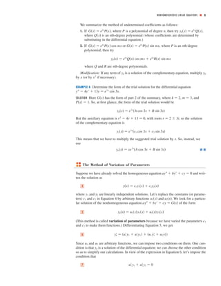
11. The solutions are all
asymptotic to as
. Except for ,
all solutions approach
either or as .
13.
15.
17.
19.
21.
23.
25.
27. y ෇ [c1 Ϫ
1
2 x ͑ex
͞x͒ dx]eϪx
ϩ [c2 ϩ
1
2 x ͑eϪx
͞x͒ dx]ex
y ෇ ͓c1 ϩ ln͑1 ϩ eϪx
͔͒ex
ϩ ͓c2 Ϫ eϪx
ϩ ln͑1 ϩ eϪx
͔͒e2x
y ෇ ͑c1 ϩ x͒ sin x ϩ ͑c2 ϩ ln cos x͒ cos x
y ෇ c1ex
ϩ c2 xex
ϩ e2x
y ෇ c1 cos 2x ϩ c2 sin 2x ϩ
1
4 x
yp ෇ xeϪx
͓͑Ax2
ϩ Bx ϩ C͒ cos 3x ϩ ͑Dx2
ϩ Ex ϩ F͒ sin 3x͔
yp ෇ Ax ϩ ͑Bx ϩ C͒e9x
yp ෇ Ae2x
ϩ ͑Bx2
ϩ Cx ϩ D͒ cos x ϩ ͑Ex2
ϩ Fx ϩ G͒ sin x
x l ϪϱϪϱϱ
ypx l ϱ
yp ෇ ex
͞10
yp
5
_4
_2 4
y ෇ ex
(1
2 x2
Ϫ x ϩ 2)
y ෇
3
2 cos x ϩ
11
2 sin x ϩ
1
2 ex
ϩ x3
Ϫ 6x
y ෇ e2x
͑c1 cos x ϩ c2 sin x͒ ϩ
1
10 eϪx
y ෇ c1 ϩ c2e2x
ϩ
1
40 cos 4x Ϫ
1
20 sin 4x
y ෇ c1eϪ2x
ϩ c2eϪx
ϩ
1
2 x2
Ϫ
3
2 x ϩ
7
4
Click here for solutions.S

1. The auxiliary equation is r2
+ 3r + 2 = (r + 2)(r + 1) = 0, so the complementary solution is
yc(x) = c1e−2x
+ c2e−x
. We try the particular solution yp(x) = Ax2
+ Bx + C, so y0
p = 2Ax + B and
y00
p = 2A. Substituting into the differential equation, we have (2A) + 3(2Ax + B) + 2(Ax2
+ Bx + C) = x2
or
2Ax2
+ (6A + 2B)x + (2A + 3B + 2C) = x2
. Comparing coefﬁcients gives 2A = 1, 6A + 2B = 0, and
2A + 3B + 2C = 0, so A = 1
2
, B = −3
2
, and C = 7
4
. Thus the general solution is
y(x) = yc(x) + yp(x) = c1e−2x
+ c2e−x
+ 1
2
x2
− 3
2
x + 7
4
.
− 2r = r(r − 2) = 0, so the complementary solution is yc(x) = c1 + c2e2x
. Try the
particular solution yp(x) = A cos 4x + B sin 4x, so y0
p = −4A sin 4x + 4B cos 4x
and y00
p = −16A cos 4x − 16B sin 4x. Substitution into the differential equation
gives (−16A cos 4x − 16B sin 4x) − 2(−4A sin 4x + 4B cos 4x) = sin 4x ⇒
(−16A − 8B) cos 4x + (8A − 16B) sin 4x = sin 4x. Then −16A − 8B = 0 and 8A − 16B = 1 ⇒ A = 1
40
and B = − 1
20
. Thus the general solution is y(x) = yc(x) + yp(x) = c1 + c2e2x
+ 1
40
cos 4x − 1
20
sin 4x.
− 4r + 5 = 0 with roots r = 2 ± i, so the complementary solution is
yc(x) = e2x
(c1 cos x + c2 sin x). Try yp (x) = Ae−x
, so y0
p = −Ae−x
and y00
p = Ae−x
. Substitution gives
Ae−x
− 4(−Ae−x
) + 5(Ae−x
) = e−x
⇒ 10Ae−x
= e−x
⇒ A = 1
10
. Thus the general solution is
y(x) = e2x
(c1 cos x + c2 sin x) + 1
10
e−x
.
+ 1 = 0 with roots r = ±i, so the complementary solution is
yc(x) = c1 cos x + c2 sin x. For y00
+ y = ex
try yp1 (x) = Aex
. Then y0
p1
= y00
p1
= Aex
and substitution gives
Aex
+ Aex
= ex
⇒ A = 1
2 , so yp1 (x) = 1
2 ex
. For y00
+ y = x3
try yp2 (x) = Ax3
+ Bx2
+ Cx + D.
Then y0
p2
= 3Ax2
+ 2Bx + C and y00
p2
= 6Ax + 2B. Substituting, we have
6Ax + 2B + Ax3
+ Bx2
+ Cx + D = x3
, so A = 1, B = 0, 6A + C = 0 ⇒ C = −6, and 2B + D = 0
⇒ D = 0. Thus yp2 (x) = x3
− 6x and the general solution is
y(x) = yc(x) + yp1 (x) + yp2 (x) = c1 cos x + c2 sin x + 1
2 ex
+ x3
− 6x. But 2 = y(0) = c1 + 1
2 ⇒ c1 = 3
2
and 0 = y0
(0) = c2 + 1
2
− 6 ⇒ c2 = 11
2
. Thus the solution to the initial-value problem is
y(x) = 3
2
cos x + 11
2
sin x + 1
2
ex
+ x3
− 6x.
− r = 0 with roots r = 0, r = 1 so the complementary solution is yc(x) = c1 + c2ex
.
Try yp(x) = x(Ax + B)ex
so that no term in yp is a solution of the complementary equation. Then
y0
p = (Ax2
+ (2A + B)x + B)ex
and y00
p = (Ax2
+ (4A + B)x + (2A + 2B))ex
. Substitution into the
differential equation gives (Ax2
+ (4A + B)x + (2A + 2B))ex
− (Ax2
+ (2A + B)x + B)ex
= xex
⇒
(2Ax + (2A + B))ex
= xex
⇒ A = 1
2
, B = −1. Thus yp(x) =
¡1
2
x2
− x
¢
ex
y(x) = c1 + c2ex
+
¡1
2
x2
− x
¢
ex
. But 2 = y(0) = c1 + c2 and 1 = y0
(0) = c2 − 1, so c2 = 2 and c1 = 0. The
solution to the initial-value problem is y(x) = 2ex
+
¡1
2
x2
− x
¢
ex
= ex
¡ 1
2
x2
− x + 2
¢
.
Solutions: Nonhomogeneous Linear Equations

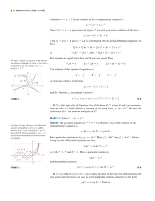
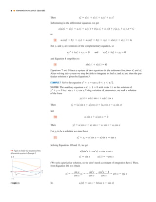
11. yc(x) = c1e−x/4
+ c2e−x
. Try yp(x) = Aex
. Then
10Aex
= ex
, so A = 1
10
y(x) = c1e−x/4
+ c2e−x
+ 1
10
ex
. The solutions are all composed
of exponential curves and with the exception of the particular
solution (which approaches 0 as x → −∞), they all approach
either ∞ or −∞ as x → −∞. As x → ∞, all solutions are
asymptotic to yp = 1
10
ex
.
13. Here yc(x) = c1 cos 3x + c2 sin 3x. For y00
+ 9y = e2x
try yp1 (x) = Ae2x
and for y00
+ 9y = x2
sin x try
yp2 (x) = (Bx2
+ Cx + D) cos x + (Ex2
+ Fx + G) sin x. Thus a trial solution is
yp(x) = yp1 (x) + yp2 (x) = Ae2x
+ (Bx2
+ Cx + D) cos x + (Ex2
+ Fx + G) sin x.
15. Here yc(x) = c1 + c2e−9x
. For y00
+ 9y0
= 1 try yp1 (x) = Ax (since y = A is a solution to the complementary
equation) and for y00
+ 9y0
= xe9x
try yp2 (x) = (Bx + C)e9x
.
17. Since yc(x) = e−x
(c1 cos 3x + c2 sin 3x) we try
yp(x) = x(Ax2
+ Bx + C)e−x
cos 3x + x(Dx2
+ Ex + F)e−x
sin 3x (so that no term of yp is a solution of the
complementary equation).
Note: Solving Equations (7) and (9) in The Method of Variation of Parameters gives
u0
1 = −
Gy2
a (y1y0
2 − y2y0
1)
and u0
2 =
Gy1
a (y1y0
2 − y2y0
1)
We will use these equations rather than resolving the system in each of the remaining exercises in this section.
19. (a) The complementary solution is yc(x) = c1 cos 2x + c2 sin 2x. A particular solution is of the form
yp(x) = Ax + B. Thus, 4Ax + 4B = x ⇒ A = 1
4
and B = 0 ⇒ yp(x) = 1
4
x. Thus, the general
solution is y = yc + yp = c1 cos 2x + c2 sin 2x + 1
4
x.
(b) In (a), yc(x) = c1 cos 2x + c2 sin 2x, so set y1 = cos 2x, y2 = sin 2x. Then
y1y0
2 − y2y0
1 = 2 cos2
2x + 2 sin2
2x = 2 so u0
1 = −1
2
x sin 2x ⇒
u1(x) = −1
2
R
x sin 2x dx = −1
4
¡
−x cos 2x + 1
2
sin 2x
¢
[by parts] and u0
2 = 1
2
x cos 2x
⇒ u2(x) = 1
2
R
x cos 2xdx = 1
4
¡
x sin 2x + 1
2
cos 2x
¢
[by parts]. Hence
yp(x) = −1
4
¡
−x cos 2x + 1
2
sin 2x
¢
cos 2x + 1
4
¡
x sin 2x + 1
2
cos 2x
¢
sin 2x = 1
4
x. Thus
y(x) = yc(x) + yp(x) = c1 cos 2x + c2 sin 2x + 1
4
x.
21. (a) r2
− r = r(r − 1) = 0 ⇒ r = 0, 1, so the complementary solution is yc(x) = c1ex
+ c2xex
. A particular
solution is of the form yp(x) = Ae2x
. Thus 4Ae2x
− 4Ae2x
+ Ae2x
= e2x
⇒ Ae2x
= e2x
⇒ A = 1
⇒ yp(x) = e2x
. So a general solution is y(x) = yc(x) + yp(x) = c1ex
+ c2xex
+ e2x
.
(b) From (a), yc(x) = c1ex
+ c2xex
, so set y1 = ex
, y2 = xex
. Then, y1y0
2 − y2y0
1 = e2x
(1 + x) − xe2x
= e2x
and so u0
1 = −xex
⇒ u1 (x) = −
R
xex
dx = −(x − 1)ex
[by parts] and u0
2 = ex
⇒
u2(x) =
R
ex
dx = ex
. Hence yp (x) = (1 − x)e2x
+ xe2x
= e2x
y(x) = yc(x) + yp(x) = c1ex
+ c2xex
+ e2x
.

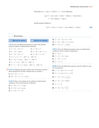
23. As in Example 6, yc(x) = c1 sin x + c2 cos x, so set y1 = sin x, y2 = cos x. Then
y1y0
2 − y2y0
1 = − sin2
x − cos2
x = −1, so u0
1 = −
sec x cos x
−1
= 1 ⇒ u1(x) = x and
u0
2 =
sec x sin x
−1
= − tan x ⇒ u2(x) = −
R
tan xdx = ln |cos x| = ln(cos x) on 0 < x < π
2
. Hence
yp(x) = x sin x + cos x ln(cos x) and the general solution is y(x) = (c1 + x) sin x + [c2 + ln(cos x)] cos x.
25. y1 = ex
, y2 = e2x
and y1y0
2 − y2y0
1 = e3x
. So u0
1 =
−e2x
(1 + e−x)e3x
= −
e−x
1 + e−x
and
u1(x) =
Z
−
e−x
1 + e−x
dx = ln(1 + e−x
). u0
2 =
ex
(1 + e−x)e3x
=
ex
e3x + e2x
so
u2(x) =
Z
ex
e3x + e2x
dx = ln
µ
ex
+ 1
ex
¶
− e−x
= ln(1 + e−x
) − e−x
. Hence
yp(x) = ex
ln(1 + e−x
) + e2x
[ln(1 + e−x
) − e−x
] and the general solution is
y(x) = [c1 + ln(1 + e−x
)]ex
+ [c2 − e−x
+ ln(1 + e−x
)]e2x
.
27. y1 = e−x
, y2 = ex
and y1y0
2 − y2y0
1 = 2. So u0
1 = −
ex
2x
, u0
2 =
e−x
2x
and
yp(x) = −e−x
Z
ex
2x
dx + ex
Z
e−x
2x
dx. Hence the general solution is
y(x) =
µ
c1 −
Z
ex
2x
dx
¶
e−x
+
µ
c2 +
Z
e−x
2x
dx
¶
ex
.

3c3 nonhomgen lineqns-stuhuhuhuhuhh

More Related Content

Similar to 3c3 nonhomgen lineqns-stuhuhuhuhuhh

Recently uploaded

3c3 nonhomgen lineqns-stuhuhuhuhuhh