Download to read offline
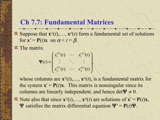
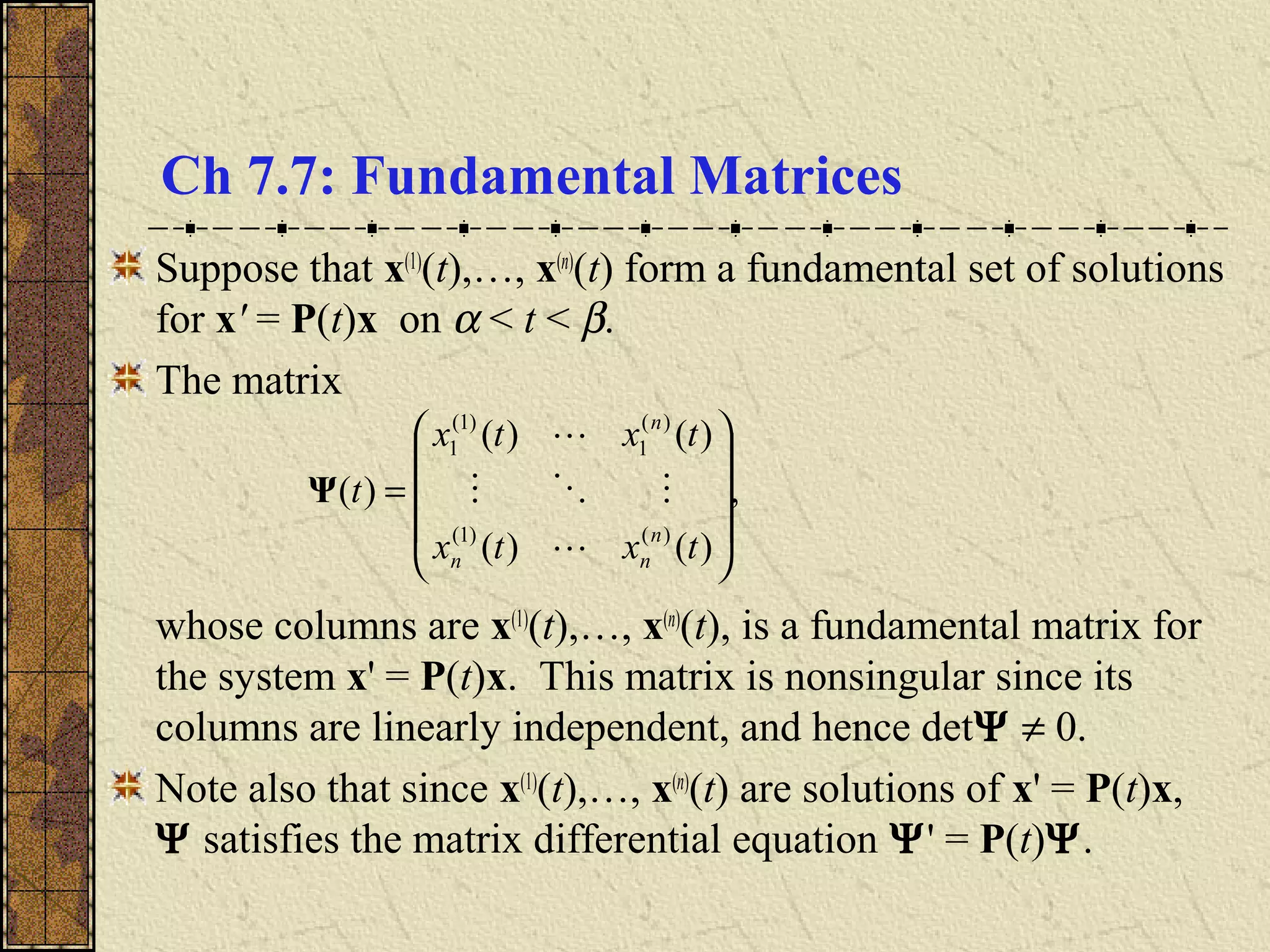
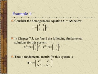
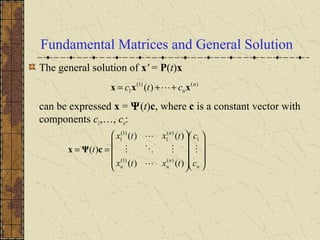
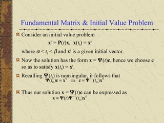
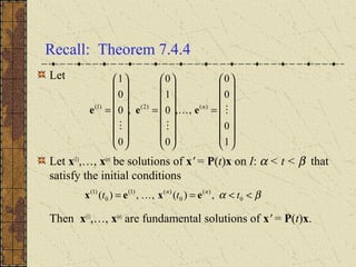
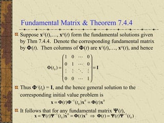
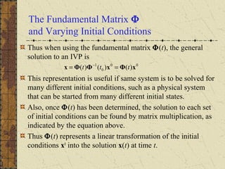
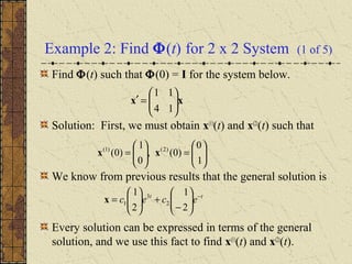
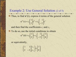
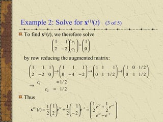
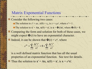
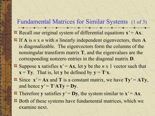

The document discusses fundamental matrices and their properties. A fundamental matrix Ψ(t) is a matrix whose columns are fundamental solutions to the system x' = P(t)x. Ψ(t) satisfies the differential equation Ψ' = P(t)Ψ and is nonsingular. The general solution to the system can be written as x = Ψ(t)c, where c is a constant vector. For an initial value problem, the solution is x = Ψ(t)Ψ-1(t0)x0. The fundamental matrix Φ(t) corresponding to a set of fundamental solutions satisfying initial conditions is also discussed. Matrix exponential functions are introduced as the fundamental matrix