Ch 5.2: Series Solutions
Near an Ordinary Point, Part I
In Chapter 3, we examined methods of solving second order
linear differential equations with constant coefficients.
We now consider the case where the coefficients are functions
of the independent variable, which we will denote by x.
It is sufficient to consider the homogeneous equation
since the method for the nonhomogeneous case is similar.
We primarily consider the case when P, Q, R are polynomials,
and hence also continuous.
However, as we will see, the method of solution is also
applicable when P, Q and R are general analytic functions.
,0)()()( 2
2
=++ yxR
dx
dy
xQ
dx
yd
xP
Ordinary Points
Assume P, Q, R are polynomials with no common factors, and
that we want to solve the equation below in a neighborhood of
a point of interest x0:
The point x0 is called an ordinary point if P(x0) ≠ 0. Since P
is continuous, P(x) ≠ 0 for all x in some interval about x0. For
x in this interval, divide the differential equation by P to get
Since p and q are continuous, Theorem 3.2.1 says there is a
unique solution, given initial conditions y(x0) = y0, y'(x0) = y0'
0)()()( 2
2
=++ yxR
dx
dy
xQ
dx
yd
xP
)(
)(
)(,
)(
)(
)(where,0)()(2
2
xP
xR
xq
xP
xQ
xpyxq
dx
dy
xp
dx
yd
===++
Singular Points
Suppose we want to solve the equation below in some
neighborhood of a point of interest x0:
The point x0 is called an singular point if P(x0) = 0.
Since P, Q, R are polynomials with no common factors, it
follows that Q(x0) ≠ 0 or R(x0) ≠ 0, or both.
Then at least one of p or q becomes unbounded as x → x0,
and therefore Theorem 3.2.1 does not apply in this situation.
Sections 5.4 through 5.8 deal with finding solutions in the
neighborhood of a singular point.
)(
)(
)(,
)(
)(
)(where,0)()(2
2
xP
xR
xq
xP
xQ
xpyxq
dx
dy
xp
dx
yd
===++
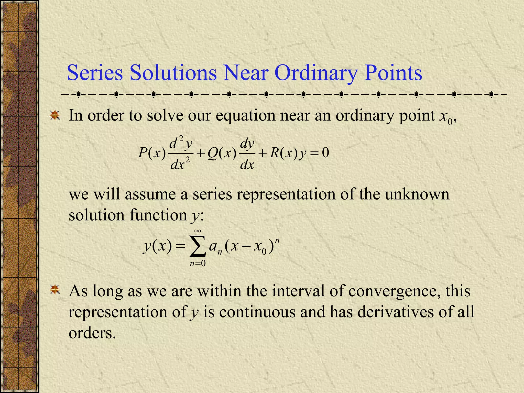
Series Solutions Near Ordinary Points
In order to solve our equation near an ordinary point x0,
we will assume a series representation of the unknown
solution function y:
As long as we are within the interval of convergence, this
representation of y is continuous and has derivatives of all
orders.
0)()()( 2
2
=++ yxR
dx
dy
xQ
dx
yd
xP
∑
∞
=
−=
0
0 )()(
n
n
n xxaxy
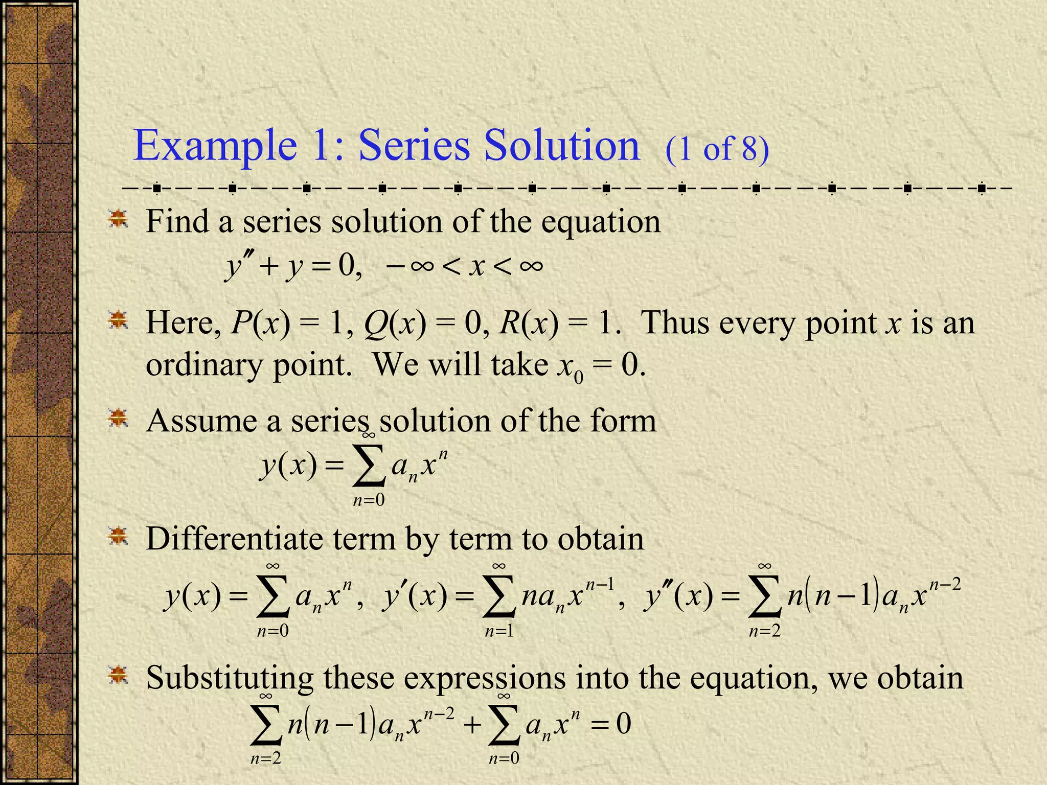
Example 1: Series Solution (1 of 8)
Find a series solution of the equation
Here, P(x) = 1, Q(x) = 0, R(x) = 1. Thus every point x is an
ordinary point. We will take x0 = 0.
Assume a series solution of the form
Differentiate term by term to obtain
Substituting these expressions into the equation, we obtain
∑
∞
=
=
0
)(
n
n
n xaxy
( )∑∑∑
∞
=
−
∞
=
−
∞
=
−=′′=′=
2
2
1
1
0
1)(,)(,)(
n
n
n
n
n
n
n
n
n xannxyxnaxyxaxy
( ) 01
02
2
=+− ∑∑
∞
=
∞
=
−
n
n
n
n
n
n xaxann
∞<<∞−=+′′ xyy ,0
Example 1: Combining Series (2 of 8)
Our equation is
Shifting indices, we obtain
( ) 01
02
2
=+− ∑∑
∞
=
∞
=
−
n
n
n
n
n
n xaxann
( )( )
( )( )[ ] 012
or
012
0
2
00
2
=+++
=+++
∑
∑∑
∞
=
+
∞
=
∞
=
+
n
n
nn
n
n
n
n
n
n
xaann
xaxann
Example 1: Recurrence Relation (3 of 8)
Our equation is
For this equation to be valid for all x, the coefficient of each
power of x must be zero, and hence
This type of equation is called a recurrence relation.
Next, we find the individual coefficients a0, a1, a2, …
( )( )
( )( )
...,2,1,0,
12
or
...,2,1,0,012
2
2
=
++
−
=
==+++
+
+
n
nn
a
a
naann
n
n
nn
( )( )[ ] 012
0
2 =+++∑
∞
=
+
n
n
nn xaann
To find a2, a4, a6, …., we proceed as follows:
Example 1: Even Coefficients (4 of 8)
( )( )12
2
++
−
=+
nn
a
a n
n
( ) ...,3,2,1,
)!2(
1
,
12345656
,
123434
,
12
0
2
04
6
02
4
0
2
=
−
=
⋅⋅⋅⋅⋅
−=
⋅
−=
⋅⋅⋅
=
⋅
−=
⋅
−=
k
k
a
a
aa
a
aa
a
a
a
k
k

To find a3, a5, a7, …., we proceed as follows:
Example: Odd Coefficients (5 of 8)
( ) ...,3,2,1,
)!12(
1
,
123456767
,
1234545
,
23
1
12
15
7
13
5
1
3
=
+
−
=
⋅⋅⋅⋅⋅⋅
−=
⋅
−=
⋅⋅⋅⋅
=
⋅
−=
⋅
−=
+ k
k
a
a
aa
a
aa
a
a
a
k
k

( )( )12
2
++
−
=+
nn
a
a n
n
Example 1: Solution (6 of 8)
We now have the following information:
Thus
Note: a0 and a1 are determined by the initial conditions.
(Expand series a few terms to see this.)
Also, by the ratio test it can be shown that these two series
converge absolutely on (-∞, ∞), and hence the
manipulations we performed on the series at each step are
11202
0 !)12(
)1(
,
!)2(
)1(
where,)( a
k
aa
k
axaxy
k
k
k
k
n
n
n
+
−
=
−
== +
∞
=
∑
12
0
1
2
0
0
!)12(
)1(
!)2(
)1(
)( +
∞
=
∞
=
∑∑ +
−
+
−
= n
n
n
n
n
n
x
n
ax
n
axy
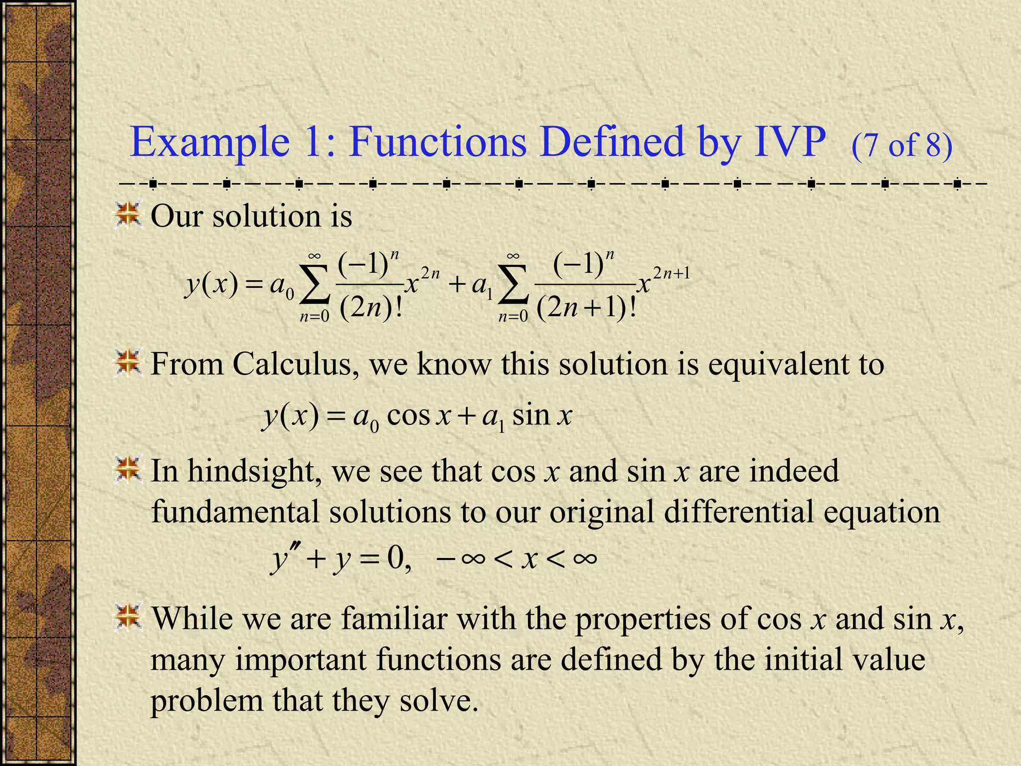
Example 1: Functions Defined by IVP (7 of 8)
Our solution is
From Calculus, we know this solution is equivalent to
In hindsight, we see that cos x and sin x are indeed
fundamental solutions to our original differential equation
While we are familiar with the properties of cos x and sin x,
many important functions are defined by the initial value
problem that they solve.
12
0
1
2
0
0
!)12(
)1(
!)2(
)1(
)( +
∞
=
∞
=
∑∑ +
−
+
−
= n
n
n
n
n
n
x
n
ax
n
axy
xaxaxy sincos)( 10 +=
∞<<∞−=+′′ xyy ,0
Example 1: Graphs (8 of 8)
The graphs below show the partial sum approximations of
cosx and sinx.
As the number of terms increases, the interval over which
the approximation is satisfactory becomes longer, and for
each x in this interval the accuracy improves.
However, the truncated power series provides only a local
approximation in the neighborhood of x = 0.
12
0
1
2
0
0
!)12(
)1(
!)2(
)1(
)( +
∞
=
∞
=
∑∑ +
−
+
−
= n
n
n
n
n
n
x
n
ax
n
axy
Example 2: Airy’s Equation (1 of 10)
Find a series solution of Airy’s equation about x0 = 0:
Here, P(x) = 1, Q(x) = 0, R(x) = - x. Thus every point x is an
ordinary point. We will take x0 = 0.
Assuming a series solution and differentiating, we obtain
Substituting these expressions into the equation, we obtain
( )∑∑∑
∞
=
−
∞
=
−
∞
=
−=′′=′=
2
2
1
1
0
1)(,)(,)(
n
n
n
n
n
n
n
n
n xannxyxnaxyxaxy
( ) 01
0
1
2
2
=−− ∑∑
∞
=
+
∞
=
−
n
n
n
n
n
n xaxann
∞<<∞−=−′′ xxyy ,0
Example 2: Combine Series (2 of 10)
Our equation is
Shifting the indices, we obtain
( ) 01
0
1
2
2
=−− ∑∑
∞
=
+
∞
=
−
n
n
n
n
n
n xaxann
( )( )
( )( )[ ] 01212
or
012
1
122
1
1
0
2
=−+++⋅⋅
=−++
∑
∑∑
∞
=
−+
∞
=
−
∞
=
+
n
n
nn
n
n
n
n
n
n
xaanna
xaxann
Example 2: Recurrence Relation (3 of 10)
Our equation is
For this equation to be valid for all x, the coefficient of each
power of x must be zero; hence a2 = 0 and
( )( )
( )( )
...,2,1,0,
23
or
,...3,2,1,
12
3
1
2
=
++
=
=
++
=
+
−
+
n
nn
a
a
n
nn
a
a
n
n
n
n
( )( )[ ] 01212
1
122 =−+++⋅⋅ ∑
∞
=
−+
n
n
nn xaanna
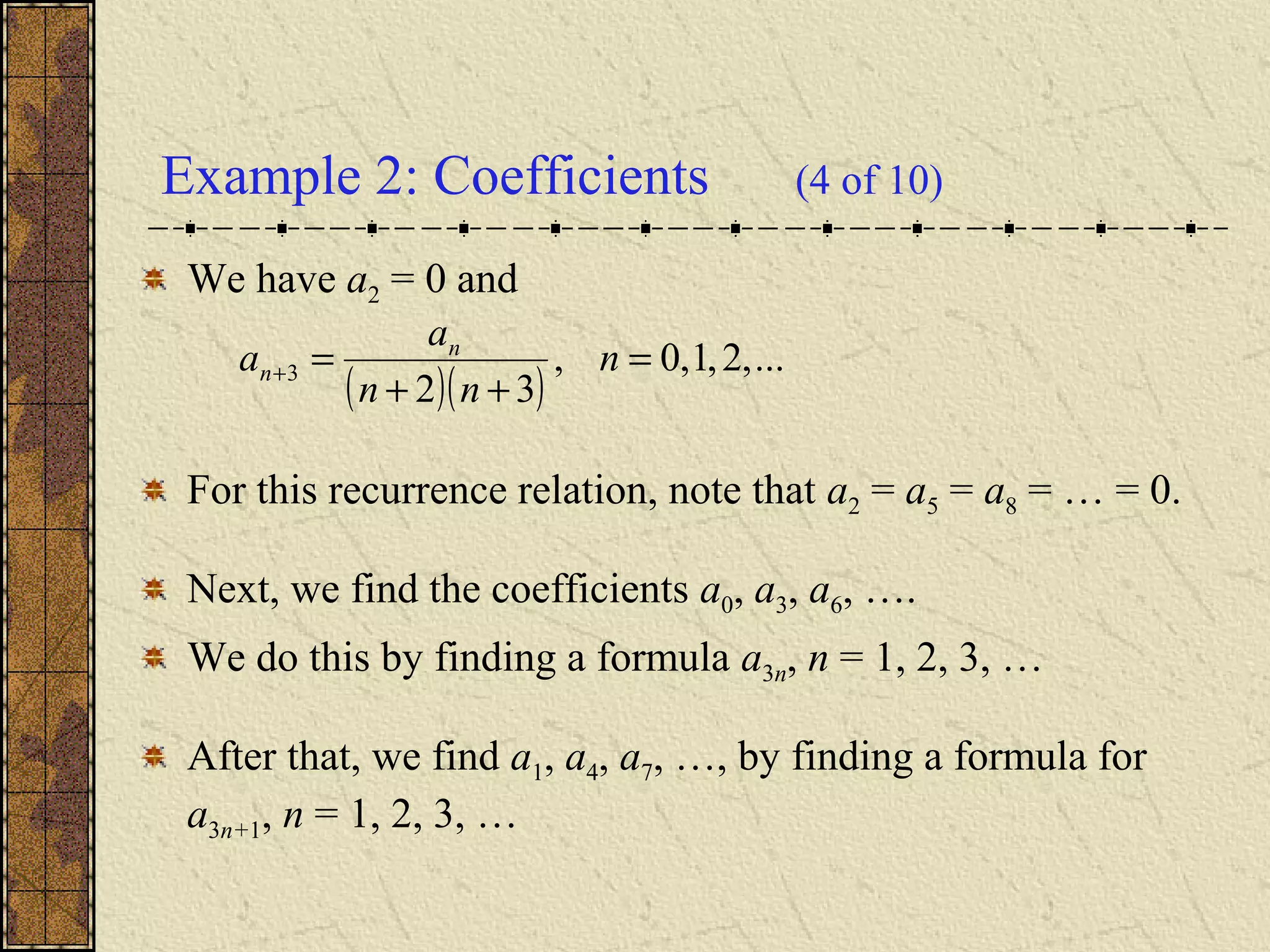
Example 2: Coefficients (4 of 10)
We have a2 = 0 and
For this recurrence relation, note that a2 = a5 = a8 = … = 0.
Next, we find the coefficients a0, a3, a6, ….
We do this by finding a formula a3n, n = 1, 2, 3, …
After that, we find a1, a4, a7, …, by finding a formula for
a3n+1, n = 1, 2, 3, …
( )( )
...,2,1,0,
32
3 =
++
=+ n
nn
a
a n
n
Example 2: Find a3n (5 of 10)
Find a3, a6, a9, ….
The general formula for this sequence is
( )( )32
3
++
=+
nn
a
a n
n
,
98653298
,
653265
,
32
06
9
03
6
0
3
⋅⋅⋅⋅⋅
=
⋅
=
⋅⋅⋅
=
⋅
=
⋅
=
aa
a
aa
a
a
a
...,2,1,
)3)(13)(33)(43(6532
0
3 =
−−−⋅⋅⋅
= n
nnnn
a
a n

Example 2: Find a3n+1 (6 of 10)
Find a4, a7, a10, …
The general formula for this sequence is
,
1097643109
,
764376
,
43
17
10
14
7
1
4
⋅⋅⋅⋅⋅
=
⋅
=
⋅⋅⋅
=
⋅
=
⋅
=
aa
a
aa
a
a
a
...,2,1,
)13)(3)(23)(33(7643
1
13 =
+−−⋅⋅⋅
=+ n
nnnn
a
a n

( )( )32
3
++
=+
nn
a
a n
n
Example 2: Series and Coefficients (7 of 10)
We now have the following information:
where a0, a1 are arbitrary, and
n
n
n
n
n
n xaxaaxaxy ∑∑
∞
=
∞
=
++==
3
10
0
)(
...,2,1,
)13)(3)(23)(33(7643
...,2,1,
)3)(13)(33)(43(6532
1
13
0
3
=
+−−⋅⋅⋅
=
=
−−−⋅⋅⋅
=
+ n
nnnn
a
a
n
nnnn
a
a
n
n


Example 2: Solution (8 of 10)
Thus our solution is
where a0, a1 are arbitrary (determined by initial conditions).
Consider the two cases
(1) a0 =1, a1 = 0 ⇔ y(0) = 1, y'(0) = 0
(2) a0 =0, a1 = 1 ⇔ y(0) = 0, y'(0) = 1
The corresponding solutions y1(x), y2(x) are linearly
independent, since W(y1, y2)(0) =1 ≠ 0, where






+⋅
++





−⋅
+= ∑∑
∞
=
+∞
= 1
13
1
1
3
0
)13)(3(43)3)(13(32
1)(
n
n
n
n
nn
x
xa
nn
x
axy

)0()0()0()0(
)0()0(
)0()0(
)0)(,( 2121
21
21
21 yyyy
yy
yy
yyW ′−′=
′′
=
Example 2: Fundamental Solutions (9 of 10)
Our solution:
For the cases
(1) a0 =1, a1 = 0 ⇔ y(0) = 1, y'(0) = 0
(2) a0 =0, a1 = 1 ⇔ y(0) = 0, y'(0) = 1,
the corresponding solutions y1(x), y2(x) are linearly
independent, and thus are fundamental solutions for Airy’s
equation, with general solution
y(x) = c1y1(x) + c1y2(x)






+⋅
++





−⋅
+= ∑∑
∞
=
+∞
= 1
13
1
1
3
0
)13)(3(43)3)(13(32
1)(
n
n
n
n
nn
x
xa
nn
x
axy

Example 2: Graphs (10 of 10)
Thus given the initial conditions
y(0) = 1, y'(0) = 0 and y(0) = 0, y'(0) = 1
the solutions are, respectively,
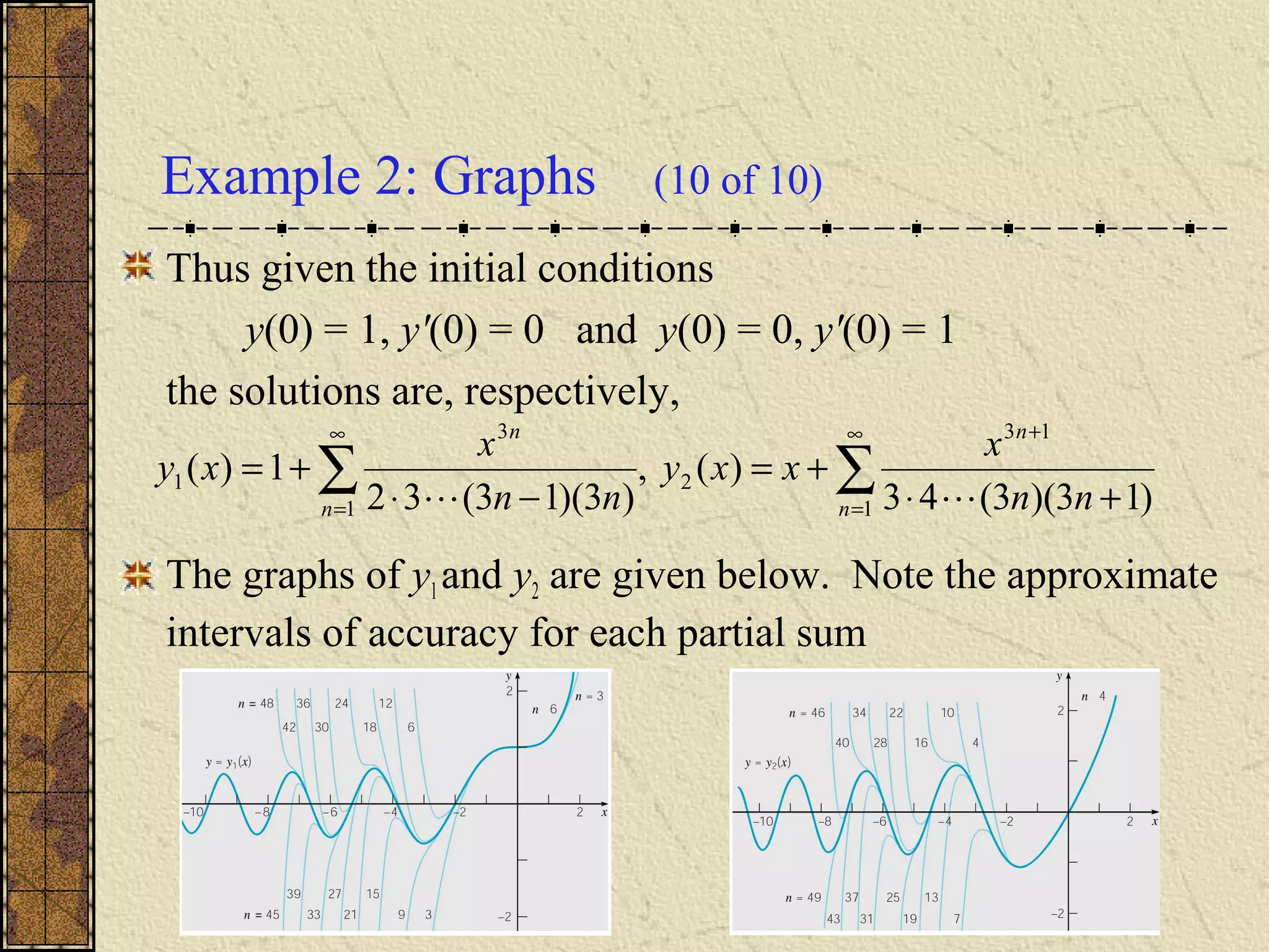
The graphs of y1and y2 are given below. Note the approximate
intervals of accuracy for each partial sum
∑∑
∞
=
+∞
= +⋅
+=
−⋅
+=
1
13
2
1
3
1
)13)(3(43
)(,
)3)(13(32
1)(
n
n
n
n
nn
x
xxy
nn
x
xy

Example 3: Airy’s Equation (1 of 7)
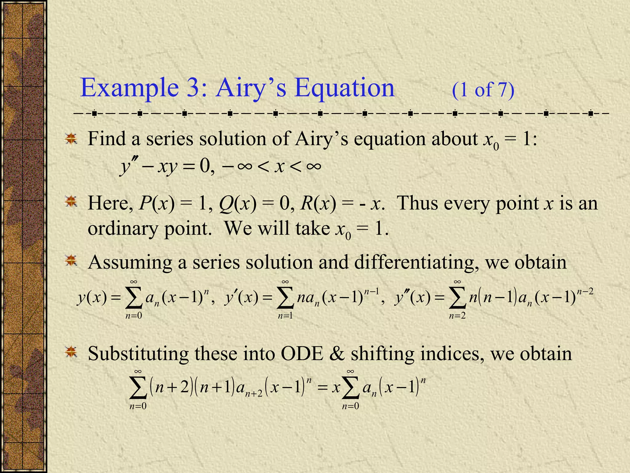
Find a series solution of Airy’s equation about x0 = 1:
Here, P(x) = 1, Q(x) = 0, R(x) = - x. Thus every point x is an
ordinary point. We will take x0 = 1.
Assuming a series solution and differentiating, we obtain
Substituting these into ODE & shifting indices, we obtain
( )∑∑∑
∞
=
−
∞
=
−
∞
=
−−=′′−=′−=
2
2
1
1
0
)1(1)(,)1()(,)1()(
n
n
n
n
n
n
n
n
n xannxyxnaxyxaxy
( )( ) ( ) ( )∑∑
∞
=
∞
=
+ −=−++
00
2 1112
n
n
n
n
n
n xaxxann
∞<<∞−=−′′ xxyy ,0
Example 3: Rewriting Series Equation (2 of
7)
Our equation is
The x on right side can be written as 1 + (x – 1); and thus
( )( ) ( ) ( )∑∑
∞
=
∞
=
+ −=−++
00
2 1112
n
n
n
n
n
n xaxxann
( )( ) ( ) [ ] ( )
( ) ( )
( ) ( )∑∑
∑∑
∑∑
∞
=
−
∞
=
∞
=
+
∞
=
∞
=
∞
=
+
−+−=
−+−=
−−+=−++
1
1
0
0
1
0
00
2
11
11
1)1(1112
n
n
n
n
n
n
n
n
n
n
n
n
n
n
n
n
n
n
xaxa
xaxa
xaxxann
Example 3: Recurrence Relation (3 of 7)
Thus our equation becomes
Thus the recurrence relation is
Equating like powers of x -1, we obtain

,
1224
34
,
66
23
,
2
2
10
4124
10
3013
0
202
aa
aaaa
aa
aaaa
a
aaa
+=⇒+=⋅
+=⇒+=⋅
=⇒=
( )( ) ( ) ( ) ( )∑∑∑
∞
=
−
∞
=
∞
=
+ −+−+=−+++
1
1
1
0
1
22 111122
n
n
n
n
n
n
n
n
n xaxaaxanna
( )( ) )1(,12 12 ≥+=++ −+ naaann nnn
Example 3: Solution (4 of 7)
We now have the following information:
and
( )∑
∞
=
−=
0
1)(
n
n
n xaxy
( ) ( ) ( )
( ) ( ) ( )






+
−
+
−
+−+






+
−
+
−
+
−
+=


12
1
6
1
1
24
1
6
1
2
1
1)(
43
1
432
0
xx
xa
xxx
axy

,
1224
,
66
,
2
arbitrary
arbitrary
10
4
10
3
0
2
1
0
aa
a
aa
a
a
a
a
a
+=
+=
=
=
=
Example 3: Solution and Recursion (5 of 7)
Our solution:
The recursion has three terms,
and determining a general formula for the coefficients an can
be difficult or impossible.
However, we can generate as many coefficients as we like,
preferably with the help of a computer algebra system.
( ) ( ) ( )
( ) ( ) ( )






+
−
+
−
+−+






+
−
+
−
+
−
+=


12
1
6
1
1
24
1
6
1
2
1
1)(
43
1
432
0
xx
xa
xxx
axy

,
1224
,
66
,
2
arbitrary
arbitrary
10
4
10
3
0
2
1
0
aa
a
aa
a
a
a
a
a
+=
+=
=
=
=
( )( ) )1(,12 12 ≥+=++ −+ naaann nnn
Example 3: Solution and Convergence (6 of 7)
Our solution:
Since we don’t have a general formula for the an, we cannot
use a convergence test (i.e., ratio test) on our power series
This means our manipulations of the power series to arrive at
our solution are suspect. However, the results of Section 5.3
will confirm the convergence of our solution.
( ) ( ) ( )
( ) ( ) ( )






+
−
+
−
+−+






+
−
+
−
+
−
+=


12
1
6
1
1
24
1
6
1
2
1
1)(
43
1
432
0
xx
xa
xxx
axy
( )∑
∞
=
−=
0
1)(
n
n
n xaxy
Example 3: Fundamental Solutions (7 of 7)
Our solution:
or
It can be shown that the solutions y3(x), y4(x) are linearly
independent, and thus are fundamental solutions for Airy’s
equation, with general solution
( ) ( ) ( )
( ) ( ) ( )






+
−
+
−
+−+






+
−
+
−
+
−
+=


12
1
6
1
1
24
1
6
1
2
1
1)(
43
1
432
0
xx
xa
xxx
axy
)()()( 4130 xyaxyaxy +=

Ch05 2

  • 1.
    Ch 5.2: SeriesSolutions Near an Ordinary Point, Part I In Chapter 3, we examined methods of solving second order linear differential equations with constant coefficients. We now consider the case where the coefficients are functions of the independent variable, which we will denote by x. It is sufficient to consider the homogeneous equation since the method for the nonhomogeneous case is similar. We primarily consider the case when P, Q, R are polynomials, and hence also continuous. However, as we will see, the method of solution is also applicable when P, Q and R are general analytic functions. ,0)()()( 2 2 =++ yxR dx dy xQ dx yd xP
  • 2.
    Ordinary Points Assume P,Q, R are polynomials with no common factors, and that we want to solve the equation below in a neighborhood of a point of interest x0: The point x0 is called an ordinary point if P(x0) ≠ 0. Since P is continuous, P(x) ≠ 0 for all x in some interval about x0. For x in this interval, divide the differential equation by P to get Since p and q are continuous, Theorem 3.2.1 says there is a unique solution, given initial conditions y(x0) = y0, y'(x0) = y0' 0)()()( 2 2 =++ yxR dx dy xQ dx yd xP )( )( )(, )( )( )(where,0)()(2 2 xP xR xq xP xQ xpyxq dx dy xp dx yd ===++
  • 3.
    Singular Points Suppose wewant to solve the equation below in some neighborhood of a point of interest x0: The point x0 is called an singular point if P(x0) = 0. Since P, Q, R are polynomials with no common factors, it follows that Q(x0) ≠ 0 or R(x0) ≠ 0, or both. Then at least one of p or q becomes unbounded as x → x0, and therefore Theorem 3.2.1 does not apply in this situation. Sections 5.4 through 5.8 deal with finding solutions in the neighborhood of a singular point. )( )( )(, )( )( )(where,0)()(2 2 xP xR xq xP xQ xpyxq dx dy xp dx yd ===++
  • 4.
    Series Solutions NearOrdinary Points In order to solve our equation near an ordinary point x0, we will assume a series representation of the unknown solution function y: As long as we are within the interval of convergence, this representation of y is continuous and has derivatives of all orders. 0)()()( 2 2 =++ yxR dx dy xQ dx yd xP ∑ ∞ = −= 0 0 )()( n n n xxaxy
  • 5.
    Example 1: SeriesSolution (1 of 8) Find a series solution of the equation Here, P(x) = 1, Q(x) = 0, R(x) = 1. Thus every point x is an ordinary point. We will take x0 = 0. Assume a series solution of the form Differentiate term by term to obtain Substituting these expressions into the equation, we obtain ∑ ∞ = = 0 )( n n n xaxy ( )∑∑∑ ∞ = − ∞ = − ∞ = −=′′=′= 2 2 1 1 0 1)(,)(,)( n n n n n n n n n xannxyxnaxyxaxy ( ) 01 02 2 =+− ∑∑ ∞ = ∞ = − n n n n n n xaxann ∞<<∞−=+′′ xyy ,0
  • 6.
    Example 1: CombiningSeries (2 of 8) Our equation is Shifting indices, we obtain ( ) 01 02 2 =+− ∑∑ ∞ = ∞ = − n n n n n n xaxann ( )( ) ( )( )[ ] 012 or 012 0 2 00 2 =+++ =+++ ∑ ∑∑ ∞ = + ∞ = ∞ = + n n nn n n n n n n xaann xaxann
  • 7.
    Example 1: RecurrenceRelation (3 of 8) Our equation is For this equation to be valid for all x, the coefficient of each power of x must be zero, and hence This type of equation is called a recurrence relation. Next, we find the individual coefficients a0, a1, a2, … ( )( ) ( )( ) ...,2,1,0, 12 or ...,2,1,0,012 2 2 = ++ − = ==+++ + + n nn a a naann n n nn ( )( )[ ] 012 0 2 =+++∑ ∞ = + n n nn xaann
  • 8.
    To find a2,a4, a6, …., we proceed as follows: Example 1: Even Coefficients (4 of 8) ( )( )12 2 ++ − =+ nn a a n n ( ) ...,3,2,1, )!2( 1 , 12345656 , 123434 , 12 0 2 04 6 02 4 0 2 = − = ⋅⋅⋅⋅⋅ −= ⋅ −= ⋅⋅⋅ = ⋅ −= ⋅ −= k k a a aa a aa a a a k k 
  • 9.
    To find a3,a5, a7, …., we proceed as follows: Example: Odd Coefficients (5 of 8) ( ) ...,3,2,1, )!12( 1 , 123456767 , 1234545 , 23 1 12 15 7 13 5 1 3 = + − = ⋅⋅⋅⋅⋅⋅ −= ⋅ −= ⋅⋅⋅⋅ = ⋅ −= ⋅ −= + k k a a aa a aa a a a k k  ( )( )12 2 ++ − =+ nn a a n n
  • 10.
    Example 1: Solution(6 of 8) We now have the following information: Thus Note: a0 and a1 are determined by the initial conditions. (Expand series a few terms to see this.) Also, by the ratio test it can be shown that these two series converge absolutely on (-∞, ∞), and hence the manipulations we performed on the series at each step are 11202 0 !)12( )1( , !)2( )1( where,)( a k aa k axaxy k k k k n n n + − = − == + ∞ = ∑ 12 0 1 2 0 0 !)12( )1( !)2( )1( )( + ∞ = ∞ = ∑∑ + − + − = n n n n n n x n ax n axy
  • 11.
    Example 1: FunctionsDefined by IVP (7 of 8) Our solution is From Calculus, we know this solution is equivalent to In hindsight, we see that cos x and sin x are indeed fundamental solutions to our original differential equation While we are familiar with the properties of cos x and sin x, many important functions are defined by the initial value problem that they solve. 12 0 1 2 0 0 !)12( )1( !)2( )1( )( + ∞ = ∞ = ∑∑ + − + − = n n n n n n x n ax n axy xaxaxy sincos)( 10 += ∞<<∞−=+′′ xyy ,0
  • 12.
    Example 1: Graphs(8 of 8) The graphs below show the partial sum approximations of cosx and sinx. As the number of terms increases, the interval over which the approximation is satisfactory becomes longer, and for each x in this interval the accuracy improves. However, the truncated power series provides only a local approximation in the neighborhood of x = 0. 12 0 1 2 0 0 !)12( )1( !)2( )1( )( + ∞ = ∞ = ∑∑ + − + − = n n n n n n x n ax n axy
  • 13.
    Example 2: Airy’sEquation (1 of 10) Find a series solution of Airy’s equation about x0 = 0: Here, P(x) = 1, Q(x) = 0, R(x) = - x. Thus every point x is an ordinary point. We will take x0 = 0. Assuming a series solution and differentiating, we obtain Substituting these expressions into the equation, we obtain ( )∑∑∑ ∞ = − ∞ = − ∞ = −=′′=′= 2 2 1 1 0 1)(,)(,)( n n n n n n n n n xannxyxnaxyxaxy ( ) 01 0 1 2 2 =−− ∑∑ ∞ = + ∞ = − n n n n n n xaxann ∞<<∞−=−′′ xxyy ,0
  • 14.
    Example 2: CombineSeries (2 of 10) Our equation is Shifting the indices, we obtain ( ) 01 0 1 2 2 =−− ∑∑ ∞ = + ∞ = − n n n n n n xaxann ( )( ) ( )( )[ ] 01212 or 012 1 122 1 1 0 2 =−+++⋅⋅ =−++ ∑ ∑∑ ∞ = −+ ∞ = − ∞ = + n n nn n n n n n n xaanna xaxann
  • 15.
    Example 2: RecurrenceRelation (3 of 10) Our equation is For this equation to be valid for all x, the coefficient of each power of x must be zero; hence a2 = 0 and ( )( ) ( )( ) ...,2,1,0, 23 or ,...3,2,1, 12 3 1 2 = ++ = = ++ = + − + n nn a a n nn a a n n n n ( )( )[ ] 01212 1 122 =−+++⋅⋅ ∑ ∞ = −+ n n nn xaanna
  • 16.
    Example 2: Coefficients(4 of 10) We have a2 = 0 and For this recurrence relation, note that a2 = a5 = a8 = … = 0. Next, we find the coefficients a0, a3, a6, …. We do this by finding a formula a3n, n = 1, 2, 3, … After that, we find a1, a4, a7, …, by finding a formula for a3n+1, n = 1, 2, 3, … ( )( ) ...,2,1,0, 32 3 = ++ =+ n nn a a n n
  • 17.
    Example 2: Finda3n (5 of 10) Find a3, a6, a9, …. The general formula for this sequence is ( )( )32 3 ++ =+ nn a a n n , 98653298 , 653265 , 32 06 9 03 6 0 3 ⋅⋅⋅⋅⋅ = ⋅ = ⋅⋅⋅ = ⋅ = ⋅ = aa a aa a a a ...,2,1, )3)(13)(33)(43(6532 0 3 = −−−⋅⋅⋅ = n nnnn a a n 
  • 18.
    Example 2: Finda3n+1 (6 of 10) Find a4, a7, a10, … The general formula for this sequence is , 1097643109 , 764376 , 43 17 10 14 7 1 4 ⋅⋅⋅⋅⋅ = ⋅ = ⋅⋅⋅ = ⋅ = ⋅ = aa a aa a a a ...,2,1, )13)(3)(23)(33(7643 1 13 = +−−⋅⋅⋅ =+ n nnnn a a n  ( )( )32 3 ++ =+ nn a a n n
  • 19.
    Example 2: Seriesand Coefficients (7 of 10) We now have the following information: where a0, a1 are arbitrary, and n n n n n n xaxaaxaxy ∑∑ ∞ = ∞ = ++== 3 10 0 )( ...,2,1, )13)(3)(23)(33(7643 ...,2,1, )3)(13)(33)(43(6532 1 13 0 3 = +−−⋅⋅⋅ = = −−−⋅⋅⋅ = + n nnnn a a n nnnn a a n n  
  • 20.
    Example 2: Solution(8 of 10) Thus our solution is where a0, a1 are arbitrary (determined by initial conditions). Consider the two cases (1) a0 =1, a1 = 0 ⇔ y(0) = 1, y'(0) = 0 (2) a0 =0, a1 = 1 ⇔ y(0) = 0, y'(0) = 1 The corresponding solutions y1(x), y2(x) are linearly independent, since W(y1, y2)(0) =1 ≠ 0, where       +⋅ ++      −⋅ += ∑∑ ∞ = +∞ = 1 13 1 1 3 0 )13)(3(43)3)(13(32 1)( n n n n nn x xa nn x axy  )0()0()0()0( )0()0( )0()0( )0)(,( 2121 21 21 21 yyyy yy yy yyW ′−′= ′′ =
  • 21.
    Example 2: FundamentalSolutions (9 of 10) Our solution: For the cases (1) a0 =1, a1 = 0 ⇔ y(0) = 1, y'(0) = 0 (2) a0 =0, a1 = 1 ⇔ y(0) = 0, y'(0) = 1, the corresponding solutions y1(x), y2(x) are linearly independent, and thus are fundamental solutions for Airy’s equation, with general solution y(x) = c1y1(x) + c1y2(x)       +⋅ ++      −⋅ += ∑∑ ∞ = +∞ = 1 13 1 1 3 0 )13)(3(43)3)(13(32 1)( n n n n nn x xa nn x axy 
  • 22.
    Example 2: Graphs(10 of 10) Thus given the initial conditions y(0) = 1, y'(0) = 0 and y(0) = 0, y'(0) = 1 the solutions are, respectively, The graphs of y1and y2 are given below. Note the approximate intervals of accuracy for each partial sum ∑∑ ∞ = +∞ = +⋅ += −⋅ += 1 13 2 1 3 1 )13)(3(43 )(, )3)(13(32 1)( n n n n nn x xxy nn x xy 
  • 23.
    Example 3: Airy’sEquation (1 of 7) Find a series solution of Airy’s equation about x0 = 1: Here, P(x) = 1, Q(x) = 0, R(x) = - x. Thus every point x is an ordinary point. We will take x0 = 1. Assuming a series solution and differentiating, we obtain Substituting these into ODE & shifting indices, we obtain ( )∑∑∑ ∞ = − ∞ = − ∞ = −−=′′−=′−= 2 2 1 1 0 )1(1)(,)1()(,)1()( n n n n n n n n n xannxyxnaxyxaxy ( )( ) ( ) ( )∑∑ ∞ = ∞ = + −=−++ 00 2 1112 n n n n n n xaxxann ∞<<∞−=−′′ xxyy ,0
  • 24.
    Example 3: RewritingSeries Equation (2 of 7) Our equation is The x on right side can be written as 1 + (x – 1); and thus ( )( ) ( ) ( )∑∑ ∞ = ∞ = + −=−++ 00 2 1112 n n n n n n xaxxann ( )( ) ( ) [ ] ( ) ( ) ( ) ( ) ( )∑∑ ∑∑ ∑∑ ∞ = − ∞ = ∞ = + ∞ = ∞ = ∞ = + −+−= −+−= −−+=−++ 1 1 0 0 1 0 00 2 11 11 1)1(1112 n n n n n n n n n n n n n n n n n n xaxa xaxa xaxxann
  • 25.
    Example 3: RecurrenceRelation (3 of 7) Thus our equation becomes Thus the recurrence relation is Equating like powers of x -1, we obtain  , 1224 34 , 66 23 , 2 2 10 4124 10 3013 0 202 aa aaaa aa aaaa a aaa +=⇒+=⋅ +=⇒+=⋅ =⇒= ( )( ) ( ) ( ) ( )∑∑∑ ∞ = − ∞ = ∞ = + −+−+=−+++ 1 1 1 0 1 22 111122 n n n n n n n n n xaxaaxanna ( )( ) )1(,12 12 ≥+=++ −+ naaann nnn
  • 26.
    Example 3: Solution(4 of 7) We now have the following information: and ( )∑ ∞ = −= 0 1)( n n n xaxy ( ) ( ) ( ) ( ) ( ) ( )       + − + − +−+       + − + − + − +=   12 1 6 1 1 24 1 6 1 2 1 1)( 43 1 432 0 xx xa xxx axy  , 1224 , 66 , 2 arbitrary arbitrary 10 4 10 3 0 2 1 0 aa a aa a a a a a += += = = =
  • 27.
    Example 3: Solutionand Recursion (5 of 7) Our solution: The recursion has three terms, and determining a general formula for the coefficients an can be difficult or impossible. However, we can generate as many coefficients as we like, preferably with the help of a computer algebra system. ( ) ( ) ( ) ( ) ( ) ( )       + − + − +−+       + − + − + − +=   12 1 6 1 1 24 1 6 1 2 1 1)( 43 1 432 0 xx xa xxx axy  , 1224 , 66 , 2 arbitrary arbitrary 10 4 10 3 0 2 1 0 aa a aa a a a a a += += = = = ( )( ) )1(,12 12 ≥+=++ −+ naaann nnn
  • 28.
    Example 3: Solutionand Convergence (6 of 7) Our solution: Since we don’t have a general formula for the an, we cannot use a convergence test (i.e., ratio test) on our power series This means our manipulations of the power series to arrive at our solution are suspect. However, the results of Section 5.3 will confirm the convergence of our solution. ( ) ( ) ( ) ( ) ( ) ( )       + − + − +−+       + − + − + − +=   12 1 6 1 1 24 1 6 1 2 1 1)( 43 1 432 0 xx xa xxx axy ( )∑ ∞ = −= 0 1)( n n n xaxy
  • 29.
    Example 3: FundamentalSolutions (7 of 7) Our solution: or It can be shown that the solutions y3(x), y4(x) are linearly independent, and thus are fundamental solutions for Airy’s equation, with general solution ( ) ( ) ( ) ( ) ( ) ( )       + − + − +−+       + − + − + − +=   12 1 6 1 1 24 1 6 1 2 1 1)( 43 1 432 0 xx xa xxx axy )()()( 4130 xyaxyaxy += )()()( 4130 xyaxyaxy +=