Downloaded 13 times
![Ch 5.7: Series Solutions
Near a Regular Singular Point, Part II
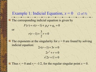
Recall from Section 5.6 (Part I): The point x0= 0 is a regular
singular point of
with
and corresponding Euler Equation
We assume solutions have the form
[ ] [ ] 0)()( 22
=+′+′′ yxqxyxxpxyx
onconvergent,)(,)(
0
2
0
ρ<== ∑∑
∞
=
∞
= n
n
n
n
n
n xxqxqxxpxxp
000
2
=+′+′′ yqyxpyx
( ) 0,0for,,)(
0
0∑
∞
=
+
>≠==
n
nr
n xaxaxrxy φ](https://image.slidesharecdn.com/ch057-150731094719-lva1-app6891/85/Ch05-7-1-320.jpg)
![Ch 5.7: Series Solutions
Near a Regular Singular Point, Part II
Recall from Section 5.6 (Part I): The point x0= 0 is a regular
singular point of
with
and corresponding Euler Equation
We assume solutions have the form
[ ] [ ] 0)()( 22
=+′+′′ yxqxyxxpxyx
onconvergent,)(,)(
0
2
0
ρ<== ∑∑
∞
=
∞
= n
n
n
n
n
n xxqxqxxpxxp
000
2
=+′+′′ yqyxpyx
( ) 0,0for,,)(
0
0∑
∞
=
+
>≠==
n
nr
n xaxaxrxy φ](https://image.slidesharecdn.com/ch057-150731094719-lva1-app6891/75/Ch05-7-1-2048.jpg)
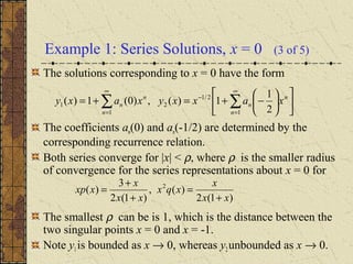
![Substitute Derivatives into ODE
Taking derivatives, we have
Substituting these derivatives into the differential equation,
we obtain
( )
( )( )∑
∑ ∑
∞
=
−+
∞
=
∞
=
−++
−++=′′
+=′=
0
2
0 0
1
1)(
,)(,)(
n
nr
n
n n
nr
n
nr
n
xnrnraxy
xnraxyxaxy
( )( )
( ) 0
1
0000
0
=
+
+
+−++
∑∑∑∑
∑
∞
=
+
∞
=
∞
=
+
∞
=
∞
=
+
n
nr
n
n
r
n
n
nr
n
n
r
n
n
nr
n
xaxqxnraxp
xnrnra
[ ] [ ] 0)()( 22
=+′+′′ yxqxyxxpxyx](https://image.slidesharecdn.com/ch057-150731094719-lva1-app6891/85/Ch05-7-2-320.jpg)
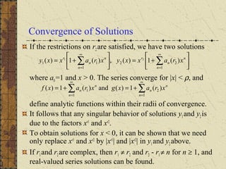
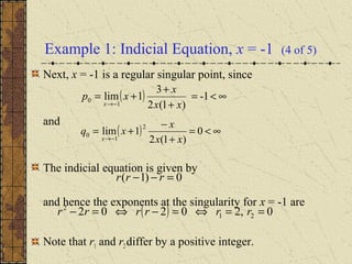
![Multiplying Series
( )
[ ] ( ) ( )[ ]
[ ] [ ]
[ ] ( )[ ]
( ) ( )[ ]
( )[ ] ( ) ( )( )[ ]
( ) ( )( ) ( )( )[ ]
+++++−++++
++++++++=
+++++++−+++
++++++++=
++++++++
+++++++++++=
+
+
+
−
+
+
−−
+
++
++
∞
=
+
∞
=
∞
=
+
∞
=
∑∑∑∑
nr
nnnn
rr
nr
nnnnnn
rr
nr
n
rrn
n
nr
n
rrn
n
n
nr
n
n
r
n
n
nr
n
n
r
n
xqnrpaqnrpaqrpa
xqrpaqrpaxqrpa
xaqaqaqrapnrapnrap
xaqaqraprapxaqrp
xaxaxaxqxqq
xnraxrarxaxpxpp
xaxqxnraxp
001110
1
001110000
01100110
1
01100110000
1
1010
1
1010
0000
1
1
1
1
1](https://image.slidesharecdn.com/ch057-150731094719-lva1-app6891/85/Ch05-7-3-320.jpg)
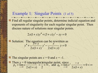
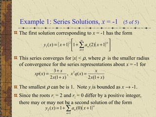
![Combining Terms in ODE
Our equation then becomes
( )( )
( )
( )( )
( )[ ] ( ) ( )( )[ ]
( ) ( )( ) ( )( )[ ]
( )[ ] ( ) ( )( )[ ]
( ) ( )( ) ( )( )[ ] 01
1)1()1(
01
1
1
0
1
000
1
001110000
001110
1
001110000
0
0000
0
=++++−++++++
++++++++++−=
=+++++−+++++
++++++++
−++=
=
+
+
+
−++
+
+
+
−
+
∞
=
+
∞
=
+
∞
=
∞
=
+
∞
=
∞
=
+
∑
∑∑∑∑
∑
nr
nnn
rr
nr
nnnn
rr
n
nr
n
n
nr
n
n
r
n
n
nr
n
n
r
n
n
nr
n
xqnrpnrnraqrpa
xqrprraqrpaxqrprra
xqnrpaqnrpaqrpa
xqrpaqrpaxqrpa
xnrnra
xaxqxnraxp
xnrnra](https://image.slidesharecdn.com/ch057-150731094719-lva1-app6891/85/Ch05-7-4-320.jpg)
![Rewriting ODE
Define F(r) by
We can then rewrite our equation
in more compact form:
( )[ ] ( ) ( )( )[ ]
( ) ( )( ) ( )( )[ ] 01
1)1()1(
000
1
001110000
=++++−+++++++
+++++++++−
+
+
nr
nnn
rr
xqnrpnrnraqrpa
xqrprraqrpaxqrprra
00)1()( qrprrrF ++−=
[ ] 0)()()(
1
1
0
0 =
+++++ +
∞
=
−
=
−∑ ∑ nr
n
n
k
kknkn
r
xqpkranrFaxrFa](https://image.slidesharecdn.com/ch057-150731094719-lva1-app6891/85/Ch05-7-5-320.jpg)
![Indicial Equation
Thus our equation is
Since a0 ≠ 0, we must have
This indicial equation is the same one obtained when
seeking solutions y = xr
to the corresponding Euler Equation.
Note that F(r) is quadratic in r, and hence has two roots,
r1 and r2. If r1 and r2 are real, then assume r1 ≥ r2.
These roots are called the exponents at the singularity, and
they determine behavior of solution near singular point.
0)1()( 00 =++−= qrprrrF
[ ] 0)()()(
1
1
0
0 =
+++++ +
∞
=
−
=
−∑ ∑ nr
n
n
k
kknkn
r
xqpkranrFaxrFa](https://image.slidesharecdn.com/ch057-150731094719-lva1-app6891/85/Ch05-7-6-320.jpg)
![Recurrence Relation
From our equation,
the recurrence relation is
This recurrence relation shows that in general, an depends on
r and the previous coefficients a0, a1, …, an-1.
Note that we must have r = r1 or r = r2.
[ ] 0)()()(
1
1
0
0 =
+++++ +
∞
=
−
=
−∑ ∑ nr
n
n
k
kknkn
r
xqpkranrFaxrFa
[ ] 0)()(
1
0
=++++ ∑
−
=
−
n
k
kknkn qpkranrFa](https://image.slidesharecdn.com/ch057-150731094719-lva1-app6891/85/Ch05-7-7-320.jpg)
![Recurrence Relation & First Solution
With the recurrence relation
we can compute a1, …, an-1 in terms of a0, pm and qm, provided
F(r + 1), F(r + 2), …, F(r + n), … are not zero.
Recall r = r1 or r = r2, and these are the only roots of F(r).
Since r1 ≥ r2, we have r1+ n ≠ r1 and r1+ n ≠ r2 for n ≥ 1.
Thus F(r1+ n) ≠ 0 for n ≥ 1, and at least one solution exists:
where the notation an(r1) indicates that an has been determined
[ ] ,0)()(
1
0
=++++ ∑
−
=
−
n
k
kknkn qpkranrFa
0,1,)(1)( 0
1
11
1
>=
+= ∑
∞
=
xaxraxxy
n
n
n
r](https://image.slidesharecdn.com/ch057-150731094719-lva1-app6891/85/Ch05-7-8-320.jpg)
![Recurrence Relation & Second Solution
Now consider r = r2. Using the recurrence relation
we compute a1, …, an-1 in terms of a0, pm and qm, provided F(r2+
1), F(r2 + 2), …, F(r2+ n), … are not zero.
If r2 ≠ r1, and r2 - r1 ≠ n for n ≥ 1, then r2+ n ≠ r1 for n ≥ 1.
Thus F(r2+ n) ≠ 0 for n ≥ 1, and a second solution exists:
where the notation an(r2) indicates that an has been determined
using r = r2.
[ ] ,0)()(
1
0
=++++ ∑
−
=
−
n
k
kknkn qpkranrFa
0,1,)(1)( 0
1
22
2
>=
+= ∑
∞
=
xaxraxxy
n
n
n
r](https://image.slidesharecdn.com/ch057-150731094719-lva1-app6891/85/Ch05-7-9-320.jpg)
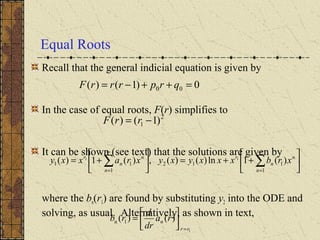
![Roots Differing by an Integer
If roots of indicial equation differ by a positive integer, i.e.,
r1 – r2 = N, it can be shown that the ODE solns are given by
where the cn(r1) are found by substituting y2 into the
differential equation and solving, as usual. Alternatively,
and
See Theorem 5.7.1 for a summary of results in this section.
++=
+= ∑∑
∞
=
∞
= 1
212
1
11 )(1ln)()(,)(1)( 21
n
n
n
r
n
n
n
r
xrcxxxayxyxraxxy
( )[ ] ,2,1,)()( 221 =−= =
nrarr
dr
d
rc rrnn
( )[ ] Nrrrarra rrN
rr
=−−= =→
212 where,)(lim 2
2](https://image.slidesharecdn.com/ch057-150731094719-lva1-app6891/85/Ch05-7-17-320.jpg)

This document discusses series solutions near regular singular points of differential equations. It begins by deriving the recurrence relation for the series coefficients from substituting a power series solution into the differential equation. It then shows how to obtain the indicial equation and exponents at the singular point. Two series solutions are given corresponding to the two exponents. An example problem finds the singular points, exponents, and series solutions for a given third order differential equation.