Download to read offline
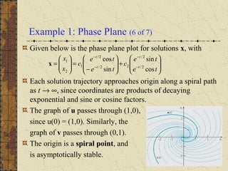
![Example 1: General Solution (5 of 7)
The corresponding solutions x = ξert
of x' = Ax are
The Wronskian of these two solutions is
Thus u(t) and v(t) are real-valued fundamental solutions of
x' = Ax, with general solution x = c1u + c2v.
=
+
=
−
=
−
=
−−
−−
t
t
ettet
t
t
ettet
tt
tt
cos
sin
cos
1
0
sin
0
1
)(
sin
cos
sin
1
0
cos
0
1
)(
2/2/
2/2/
v
u
[ ] 0
cossin
sincos
)(, 2/2/
2/2/
)2()1(
≠=
−
= −
−−
−−
t
tt
tt
e
tete
tete
tW xx](https://image.slidesharecdn.com/ch076-150731094826-lva1-app6891/85/Ch07-6-10-320.jpg)
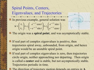
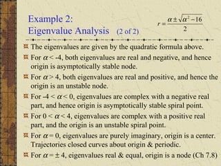

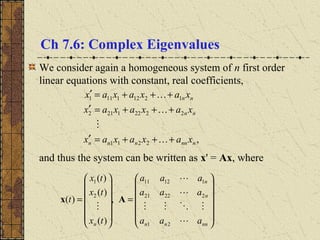
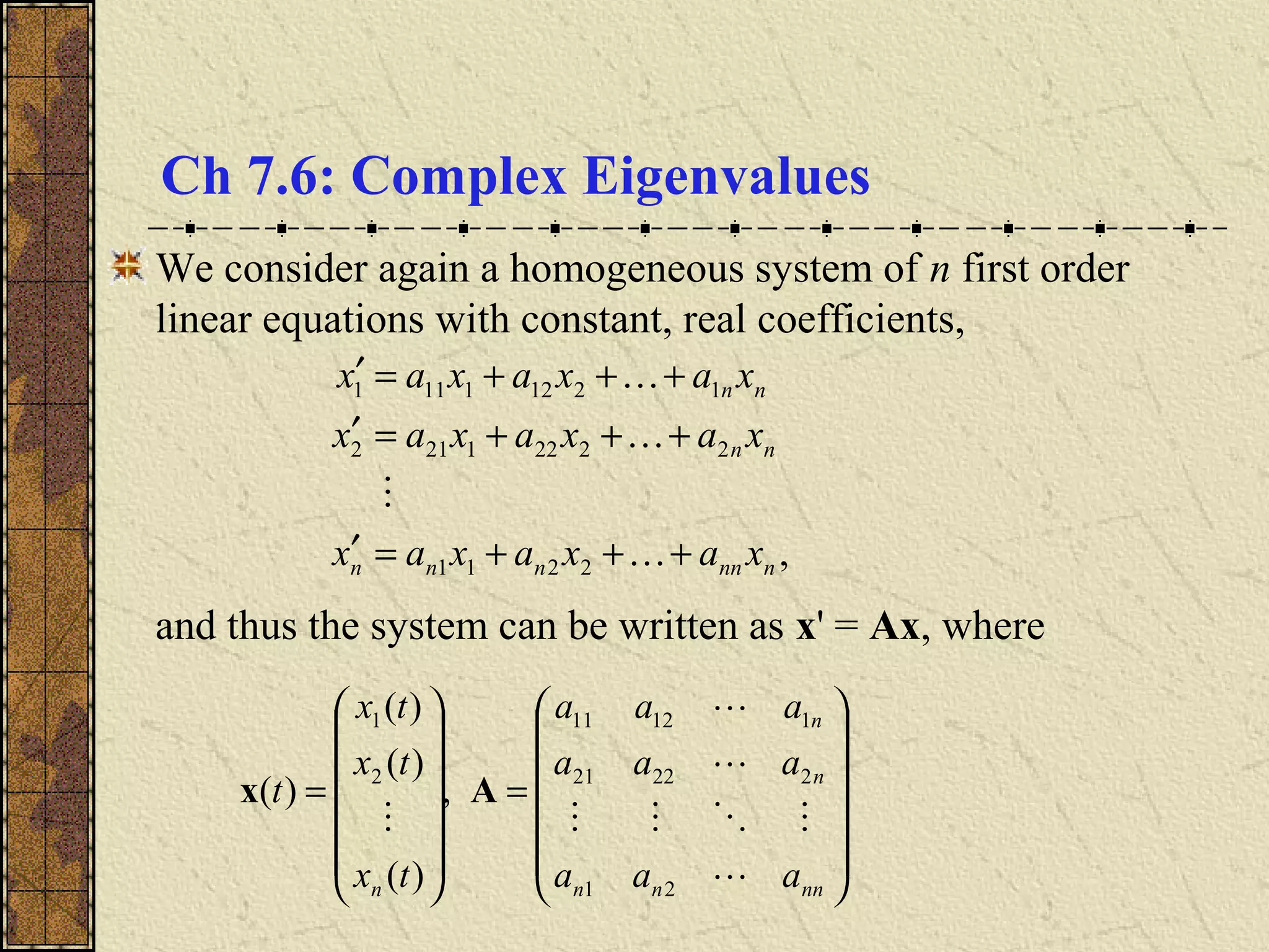
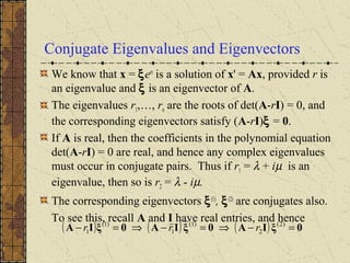
The document discusses complex eigenvalues and eigenvectors for systems of linear differential equations. It shows that if the matrix A has complex conjugate eigenvalue pairs r1 and r2, then the corresponding eigenvectors and solutions will also be complex conjugates. This leads to real-valued fundamental solutions that can express the general solution. An example demonstrates these concepts, finding the complex eigenvalues and eigenvectors and expressing the general solution in terms of real-valued functions. Spiral points, centers, eigenvalues, and trajectory behaviors are also summarized.