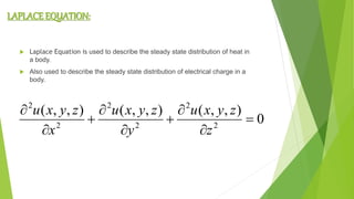
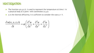
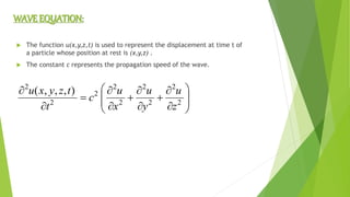
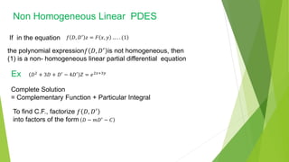
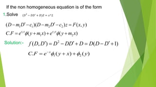
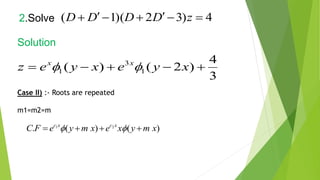
The document discusses higher-order non-homogeneous partial differential equations (PDEs), providing definitions, general forms, and methods for finding solutions. It highlights the role of complementary functions and particular integrals in obtaining complete solutions, with examples illustrating these concepts. Additionally, the applications of PDEs in various scientific fields, including heat and wave equations, are mentioned, showcasing their significance in modeling complex phenomena.

1. Name :- Vrajesh shah(150410116108)
Sub :- Advanced engineering mathematics
Topic:- Higherorder Non Homogeneous Partial
Differential Equations
Department :-IT
SARDAR VALLABHBHAI PATEL INSTITUTE OF TECHNOLOGY

2. Definition :-
A partial differential equation is an equation involving a function of
two or more variables and some of its partial derivatives. Therefore
a partial differential equation contains one dependent variable and
more than one independent variable.
Here z will be taken as the dependent variable and x and y
the independent variable so that .
We will use the following standard notations to denote the partial
derivatives.
 yxfz , .
,, q
y
z
p
x
z






t
y
z
s
yx
z
r
x
z









2
22
2
2
,,

3. Solution to non homogeneous partial
differential equation
 General Form of 2nd order Non-Homogeneous Partial differential equations :-

𝑎0𝜕2Z
𝜕x2 +
𝑎1𝜕2Z
𝜕x𝜕y
+
𝑎2𝜕2Z
𝜕y2 = 𝑓(𝑥, 𝑦)
 Where 𝑎0 , 𝑎1, 𝑎2 𝑎𝑟𝑒 𝑐𝑜𝑛𝑠𝑡𝑎𝑛𝑡𝑠

𝜕
𝜕x
= 𝐷 ;
𝜕
𝜕y
= 𝐷′
 (𝑎0𝐷2 + 𝑎1𝐷𝐷′ + 𝑎2𝐷′2)𝑍 = 𝑓(𝑥, 𝑦)
 F (D , D’) Z = f ( 𝑥 , y )
 Solution is given by Z = Complimentary Function (C.F) + Particular Integral (P.I)
 Complimentary Function (From L.H.S)
 Particular Integral (From R.H.S)

4. Non Homogeneous Linear PDES
If in the equation
the polynomial expression𝑓 𝐷, 𝐷′
is not homogeneous, then
(1) is a non- homogeneous linear partial differential equation
Complete Solution
= Complementary Function + Particular Integral
To find C.F., factorize 𝑓 𝐷, 𝐷′
into factors of the form
Ex
)𝑓 𝐷, 𝐷′
𝑧 = 𝐹 𝑥, 𝑦 … . . (1
𝐷2 + 3𝐷 + 𝐷′ − 4𝐷′ 𝑍 = 𝑒2𝑥+3𝑦
𝐷 − 𝑚𝐷′
− 𝐶

5. If the non homogeneous equation is of the form
)()(.
),())((
21
2211
21
xmyexmyeFC
yxFzcDmDcDmD
xcxc



1.Solve
Solution:- )1(),( 2
 DDDDDDDDDf
)()(. 21 yxyeFC x
  

6. 

























 





 




 




6.5.125.4.34.3123
1
......
)1()1(1
)1(
1
1
.
65443
2
2
2
2
22
2
2
1
22
2
xxxxx
x
D
x
D
D
x
D
D
x
D
x
D
D
DDDDD
x
IP

7. 2.Solve 4)32)(1(  zDDDD
Solution
3
4
)2()( 1
3
1  xyexyez xx

Case II) :- Roots are repeated
m1=m2=m
)()(. 21
xmyxexmyeFC xcxc
 

8. Rules for finding Particular Integral
 F ( D , D’ ) Z = f ( 𝑥 , y )
 Case I :- f (𝑥 , y ) = 𝑒 𝑎𝑥+𝑏𝑦
P.I =
1
f D,D’
𝑒 𝑎𝑥+𝑏𝑦
, P.I =
1
f a,b
𝑒 𝑎𝑥+𝑏𝑦
; f ( a , b ) ≠ 0
 Case II :- sin 𝑎𝑥 + 𝑏𝑦 𝑜𝑟 cos(𝑎𝑥 + 𝑏𝑦)
P.I =
1
𝑓 𝐷2,𝐷𝐷′,𝐷′2 sin 𝑎𝑥 + 𝑏𝑦
P.I =
1
𝑓 −𝑎2,−𝑎𝑏,−𝑏2 sin 𝑎𝑥 + 𝑏𝑦 , 𝑓(−𝑎2
, −𝑎𝑏, −𝑏2
) ≠ 0

9.  Case III :- 𝑓 𝑥, 𝑦 = 𝑥 𝑚 𝑦 𝑛
P.I =
1
𝑓 𝐷,𝐷′ 𝑥 𝑚 𝑦 𝑛
 If m<n then expansion is in powers of
𝐷
𝐷′
 If m>n then expansion is in powers of
𝐷′
𝐷
Use :-
1.
1
1+𝑥
= 1 − 𝑥 + 𝑥2
− ⋯
2.
1
1−𝑥
= 1 + 𝑥 + 𝑥2
+ ⋯
3. 𝐷 =
𝜕
𝜕x
;
1
𝐷
= 𝑦
𝑓 𝑥, 𝑦 𝑑𝑥
4. 𝐷′ =
𝜕
𝜕y
;
1
𝐷′ = 𝑦
𝑓 𝑥, 𝑦 𝑑𝑦

10.  Case IV (General Rule) :- (Rule for failure case )

1
𝐷−𝑚𝐷′ 𝑓 𝑥, 𝑦 = 𝑦
𝑓 𝑥, −𝑚𝑥 𝑑𝑥 −
After integration , Substitute c = y + mx

11. Example:-1
1) 𝐷2
− 2𝐷𝐷′
+ 𝐷′2
𝑍 = 0
The Auxiliary equation is given by
𝑚2
− 2𝑚 + 1 = 0
m = -1 , -1
Roots are repeated
C.F = 𝑓1 𝑦 − 𝑥 + 𝑥𝑓2 𝑦 − 𝑥
P.I = 𝐷2 − 2𝐷𝐷′ + 𝐷′2 𝑍 = 𝑒 𝑥+4𝑦
P.I =
1
𝐷2−2𝐷𝐷′+𝐷′2 𝑒 𝑥+4𝑦
P.I =
1
12−2 1 4 +42 𝑒 𝑥+4𝑦
P.I=
1
9
𝑒 𝑥 + 4𝑦
Solution is Z = C.F + P.I
Z = 𝑓1 𝑦 − 𝑥 + 𝑥𝑓2 𝑦 − 𝑥 +
1
9
𝑒 𝑥+4𝑦

12. Example :- 2
2) 𝐷2 − 𝐷𝐷′ = 𝑠𝑖𝑛𝑥𝑠𝑖𝑛2𝑦
The Auxiliary equation is given by
𝑚2
− 𝑚 = 0
m(m-1)=0
Roots are real and distinct
m=0, 1 ----ROOTS
C.F = 𝑓1 𝑦 + 𝑓2 𝑦 + 𝑥

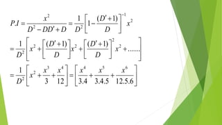
13. P.I = 𝐷2
− 𝐷𝐷′
𝑍 = −
1
2 2𝑠𝑖𝑛𝑥𝑠𝑖𝑛2𝑦
P.I= −
1
2 cos 𝑥+2𝑦 −cos 𝑥−2𝑦
P.I =
1
𝐷−𝐷𝐷′ −
1
2
cos 𝑥 + 2𝑦 − cos 𝑥1 − 2𝑦
P.I= [−
1
2
1
D2−DD’
cos 𝑥 + 2𝑦 −
1
𝐷2−𝐷𝐷′ cos 𝑥 − 2𝑦 ]
P.I= −
1
2
1
1 2− 1 2
cos 𝑥 + 2𝑦 −
1
1 2− 1 −2
cos 𝑥 − 2𝑦
P.I= −
1
2
cos 𝑥 + 2𝑦 −
1
3
cos 𝑥 − 2𝑦
P.I=
1
2
cos 𝑥 + 2𝑦 −
1
6
cos 𝑥 − 2𝑦
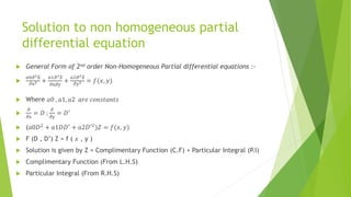
Solution is Z = C.F + P.I
 Z = 𝑓1 𝑦 + 𝑓2 𝑦 + 𝑥 +
1
2
cos 𝑥 + 2𝑦 −
1
6
cos 𝑥 − 2𝑦

14. PDEs are used to model many systems in many different fields of science
and engineering.
Important Examples:
 Laplace Equation
 Heat Equation
 Wave Equation
Application of pde:

15.  Laplace Equation is used to describe the steady state distribution of heat in
a body.
 Also used to describe the steady state distribution of electrical charge in a
body.
LAPLACE EQUATION:
0
),,(),,(),,(
2
2
2
2
2
2









z
zyxu
y
zyxu
x
zyxu

16.  The function u(x,y,z,t) is used to represent the temperature at time t in
a physical body at a point with coordinates (x,y,z)
  is the thermal diffusivity. It is sufficient to consider the case  = 1.
HEAT EQUATION:

















2
2
2
2
2
2
),,,(
z
u
y
u
x
u
t
tzyxu


17.  The function u(x,y,z,t) is used to represent the displacement at time t of
a particle whose position at rest is (x,y,z) .
 The constant c represents the propagation speed of the wave.
WAVE EQUATION:



















2
2
2
2
2
2
2
2
2
),,,(
z
u
y
u
x
u
c
t
tzyxu

18.  PDEs can be used to describe a wide variety of phenomena
such as sound, heat, electrostatics, electrodynamics, fluid
dynamics, elasticity, or quantum mechanics. These
seemingly distinct physical phenomena can be formalised
similarly in terms of PDEs. Just as ordinary differential
equations often model one-dimensional dynamical
systems, partial differential equations often
model multidimensional systems. PDEs find their
generalisation instochastic partial differential equations.
APPLICATIONS

19. THANK YOU