Download to read offline
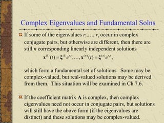
![Example 1: General Solution (5 of 9)
The corresponding solutions x = ξert
of x' = Ax are
The Wronskian of these two solutions is
Thus x(1)
and x(2)
are fundamental solutions, and the general
solution of x' = Ax is
tt
etet −
−
=
=
2
1
)(,
2
1
)( )2(3)1(
xx
[ ] 04
22
)(, 2
3
3
)2()1(
≠−=
−
= −
−
−
t
tt
tt
e
ee
ee
tW xx
tt
ecec
tctct
−
−
+
=
+=
2
1
2
1
)()()(
2
3
1
)2(
2
)1(
1 xxx](https://image.slidesharecdn.com/ch075-150731094817-lva1-app6892/85/Ch07-5-9-320.jpg)
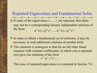
![Example 2: General Solution (5 of 9)
The corresponding solutions x = ξert
of x' = Ax are
The Wronskian of these two solutions is
Thus x(1)
and x(2)
are fundamental solutions, and the general
solution of x' = Ax is
tt
etet 4)2()1(
1
2
)(,
2
1
)( −−
−
=
= xx
[ ] 03
2
2
)(, 5
4
4
)2()1(
≠=
−
= −
−−
−−
t
tt
tt
e
ee
ee
tW xx
tt
ecec
tctct
4
21
)2(
2
)1(
1
1
2
2
1
)()()(
−−
−
+
=
+= xxx](https://image.slidesharecdn.com/ch075-150731094817-lva1-app6892/85/Ch07-5-18-320.jpg)
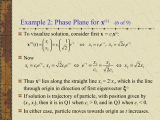
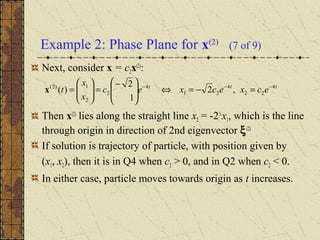
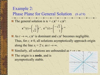
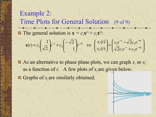
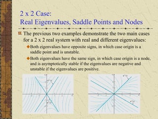
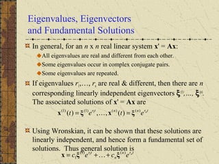
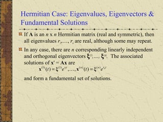
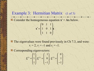

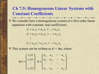
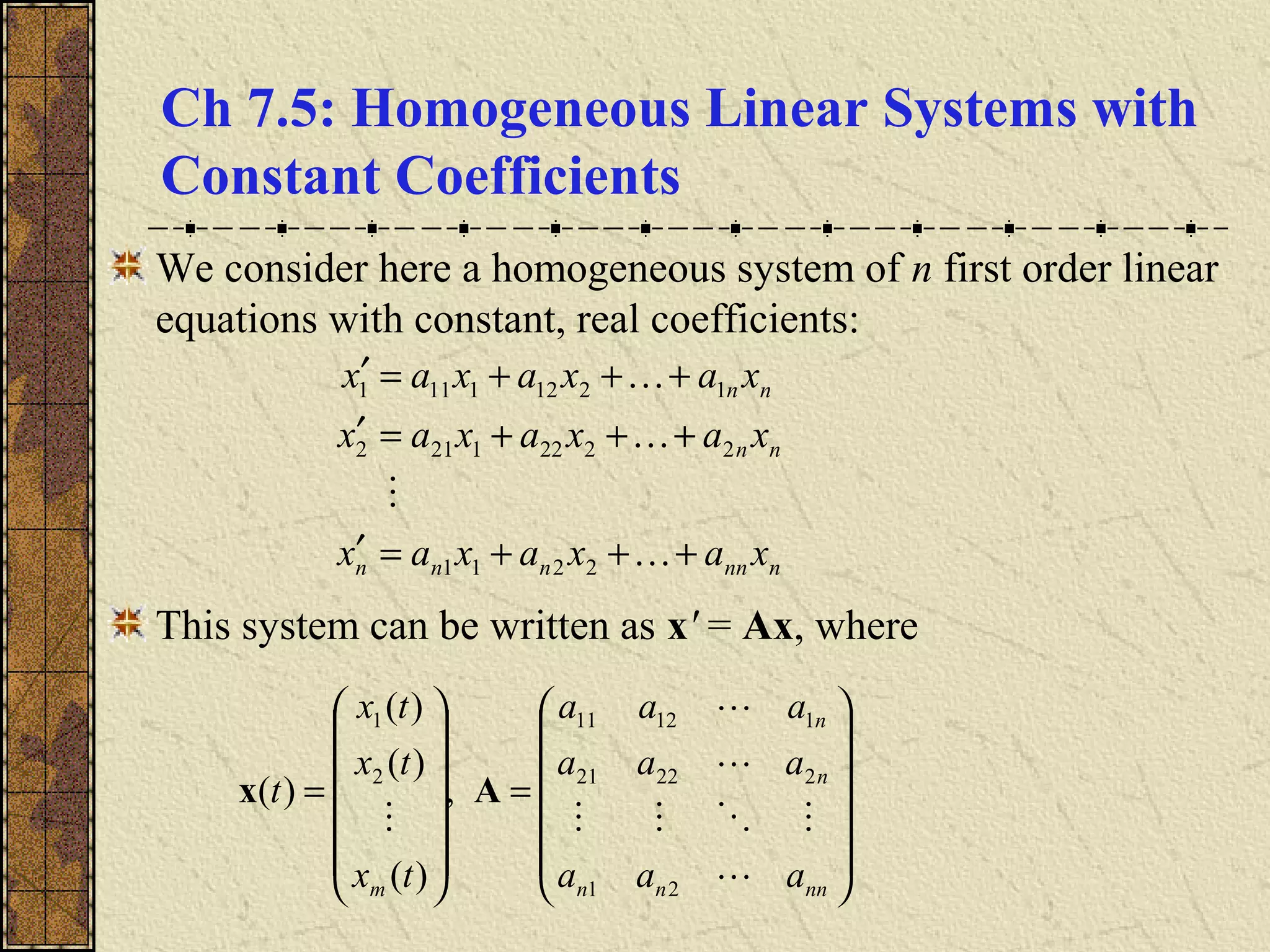
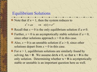
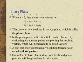
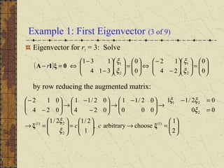
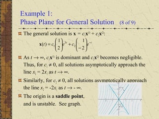
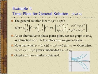
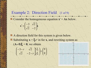
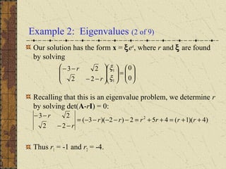
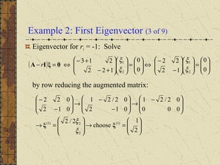
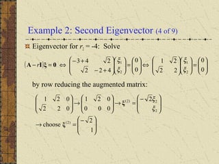
This document discusses homogeneous linear systems with constant coefficients. It begins by defining such a system as x' = Ax, where A is an n×n matrix of real constants. It then explains that the equilibrium solutions are found by solving Ax = 0, and stability is determined by the eigenvalues of A. Examples are provided to illustrate finding the direction field, eigenvalues/eigenvectors, general solution, and phase plane plots for specific 2D systems. Time plots of the solutions are also shown.


![Week 8 [compatibility mode]](https://cdn.slidesharecdn.com/ss_thumbnails/week8compatibilitymode-130213163443-phpapp01-thumbnail.jpg?width=640&height=640&fit=bounds)