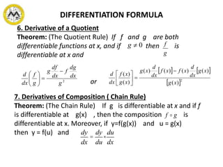
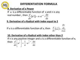
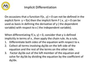
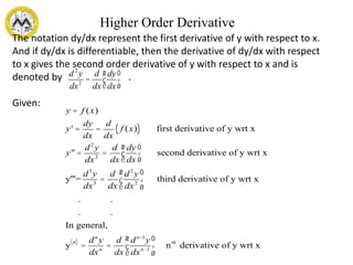
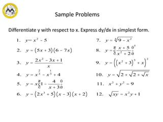
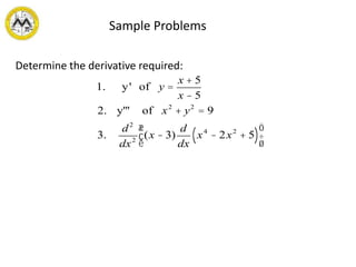
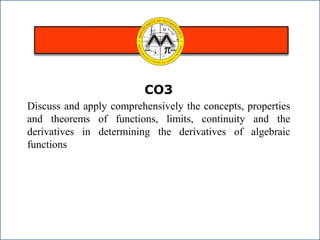
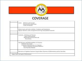
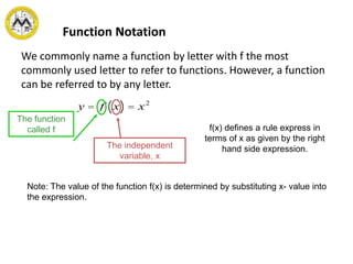
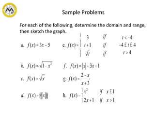
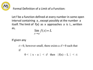
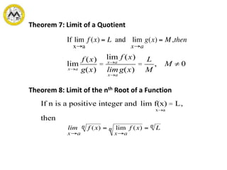
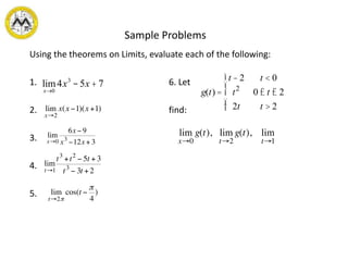
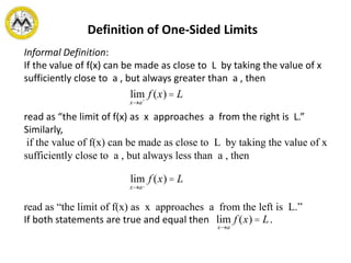
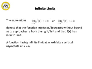
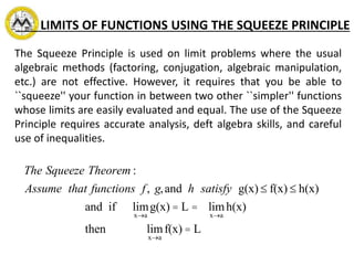
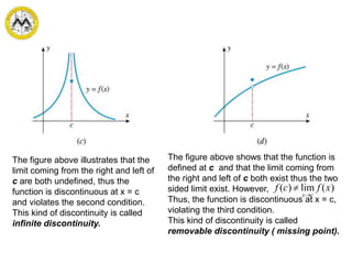
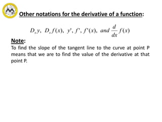
This document discusses concepts related to calculus including limits, continuity, and derivatives of functions. Specifically, it covers: - Definitions and theorems related to limits, continuity, and derivatives of algebraic functions. - Evaluating limits, determining continuity of functions, and taking derivatives of algebraic functions using basic theorems of differentiation. - The objective is for students to be able to evaluate limits, determine continuity, and find derivatives of continuous algebraic functions in explicit or implicit form after discussing these calculus concepts.

1. CO3
Discuss and apply comprehensively the concepts, properties
and theorems of functions, limits, continuity and the
derivatives in determining the derivatives of algebraic
functions

2. COVERAGE
Limits: Definition and Concepts
Theorems One-Sided Limits
Limits of Functions
Infinite Limits and Limits at Infinity: Evaluation and Interpretation
Squeeze Theorem: Limits of Expression Involving Transcendental Functions
Continuity : Definition and Theorem
Types of Discontinuity;
Relationship between limits and
Discontinuity
The Derivative and Differentiability of a Function:
Definition and concept
Evaluation of the Derivative of a Function
based on Definition (Increment Method or
Four-Step Rule Method)
Derivatives of Algebraic Functions Using the Basic Theorems of Differentiation and the Chain Rule
Higher Order and Implicit Differentiation

3. Objective:
At the end of the discussion, the students
should be able to evaluate limits and determine
the derivative of a continuous algebraic function
given in the explicit or implicit form.

4. The Calculus

5. Calculus
- Is the mathematics of change
- two basic branches: differential and integral
calculus

6. Lesson 1 : Functions and Limits

7. FUNCTIONS
- A relation between variables x and y is a rule of
correspondence that assigns an element x from the Set A to
an element y of Set B.
- A function f from set A to set B is a rule of correspondence
that assigns to each element x in the set A exactly one
element y in the set B. It is a set of ordered pairs ( x, y) such
that no two pairs will have the same first element.

8. Domain (set of all x’s) Range (set of all y’s)
1
2
3
4
5
2
10
8
6
4
Mapping of X- values into y-values ( 1 -1 correspendence)
X Y

9. X = Set A
Domain Set
1
2
3
4
5
Y = Set B
Range Set
2
10
8
6
4
Mapping illustrating many – 1 correspondence

10. 1
2
3
4
5
2
10
8
6
4
Mapping of the elements of Set A in to Set B illustrating 1 – many type
of correspondence.
X = Set A Y = Set B

11. Function Notation
We commonly name a function by letter with f the most
commonly used letter to refer to functions. However, a function
can be referred to by any letter.
y = f x( ) = x2
The function
called f
The independent
variable, x
f(x) defines a rule express in
terms of x as given by the right
hand side expression.
Note: The value of the function f(x) is determined by substituting x- value into
the expression.

12. PIECEWISE DEFINED FUNCTION
A piecewise defined function is function defined by different
formulas on different parts of its domain; as in,
f (x) =
2x2
+3
5x -1
ì
í
î
if x<0
if x ³ 0
g(x) = x =
x
-x
if
if
x ³ 0
x < 0
ì
í
ï
îï

13. Graph of a Function
The graph of a function f consists of all points (x, y) whose
coordinates satisfy y = f(x), for all x in the domain of f. The set of
ordered pairs (x, y) may also be represented by (x, f(x)) since y = f(x).
Recall: The Vertical Line Test
A set of points in a coordinate plane is the graph of a
function y = f(x) if and only if no vertical line intersects the graph at
more than one point.

14. ODD and EVEN FUNCTIONS
A function is an even function if and only if
The graph of an even function is
symmetric with respect to the y-axis.
A function is an odd function if and only if
The graph of an odd function is
symmetric with respect to the origin.
y = f (x)
f (-x) = f (x).
y = f (x)
f (-x) = - f (x).

15. Sample Problems
For each of the following, determine the domain and range,
then sketch the graph.
a. f(x)=3x-5 e. f(x)=
3
t+1
t
ì
í
ï
î
ï
if
if
if
t <-4
-4 £t £ 4
t > 4
b. f(x)= 1- x2
f. f(x)= x +3x+1
c. f(x)= x g. f(x)=
2- x
x+3
d. f(x)= xéë ùû h. f(x)=
x2
if x £1
2x+1 if x >1
ì
í
î

16. with domain the set of all x in the domain of g such that g(x) is
in the domain of f or in other words, whenever both g(x) and
f(g(x)) are defined.
In the same way,
with domain as the set of all x in the domain of f such that f(x)
is in the domain of g, or, in other words, whenever both f(x)
and g(f(x)) are defined.
The composition function, denoted by , is defined asf g
f g = f (g(x))
g f = g( f(x))

17. For each of the following pair of functions:
a) f(x) = 2x – 5 and g(x) = x2 – 1
b) and
determine the following functions:
a) f + g b) f - g c) fg d) f/g e) g/f
f)
g) domain of each resulting functions.
Sample Problems
f g, and g f
g(x)= x-1f (x) =
2
x

18. Informal Definition: If the values of f(x) can be made as
close as possible to some value L by taking the value of x
as close as possible, but not equal to, a, then we write
Read as “ the limit of f(x) as x approaches a is L” or
“ f(x) approaches L as x approaches a”. This can also be
written as
lim
x®a
f (x) = L
f (x)® L as x ® a.

19. Formal Definition of a Limit of a Function:
Let f be a function defined at every number in some open
interval containing a , except possibly at the number a
itself. The limit of f(x) as x approaches a is L , written
as,
If given any
e > 0, however small, there exists a d > 0 such that
if
0 < | x - a | < d then | f(x) - L | < e.

20. Geometrically, this can be viewed as follows:

21. Theorem 1: Limit of a Constant
If c is a constant, then for any number a
Theorem 2: Limit of the Identify Function
Theorem 3: Limit of a Linear Function
If m and b are constants
Theorem 4: Limit of the Sum or Difference of Functions
lim
x®a
(mx + b) = ma + b

22. Theorem 5: Limit of the Product
Theorem 6: Limit of the nth Power of a function
Iflimf(x)=L
x®a
andnisanypositiveinteger,then

23. Theorem 7: Limit of a Quotient
Theorem 8: Limit of the nth Root of a Function
lim
x®a
f (x)
g(x)
=
lim
x®a
f (x)
lim
x®a
g(x)
=
L
M
, M ¹ 0
If n is a positive integer and lim f(x) = L
x®a
,
then

24. Using the theorems on Limits, evaluate each of the following:
1. 6. Let
2. find:
3.
4.
5.
g(t) =
t - 2 t < 0
t2
0 £ t £ 2
2t t > 2
ì
í
ï
î
ï
Sample Problems
lim
x®0
4x3
-5x + 7

25. Definition of One-Sided Limits
Informal Definition:
If the value of f(x) can be made as close to L by taking the value of x
sufficiently close to a , but always greater than a , then
read as “the limit of f(x) as x approaches a from the right is L.”
Similarly,
if the value of f(x) can be made as close to L by taking the value of x
sufficiently close to a , but always less than a , then
read as “the limit of f(x) as x approaches a from the left is L.”
If both statements are true and equal then .
lim
x®a+
f (x) = L
lim
x®a_
f (x) = L
lim
x®a
f (x) = L

26. Geometrically,

29. Infinite Limits
The expressions
denote that the function increases/decreases without bound
as x approaches a from the right/ left and that f(x) has
infinite limit.
A function having infinite limit at a exhibits a vertical
asymptote at x = a.
lim
x®a+
f (x)®±¥ or lim
x®a-
f (x)®±¥

31. x=a
0
x=a
0
Geometrically;

32. Limits at Infinity
If as x increases/decreases without bound, the value of the
function f(x) gets closer and closer to L then
If L is finite, then limits at infinity is associated with the existence
of a horizontal asymptote at y = L.
lim
x®¥
f (x) = L or lim
x®-¥
f (x) = L.

33. Geometrically,

34. Y=L
0
Y=L
lim
x®+¥
f (x) = L
0
lim
x®+¥
f (x) = L

35. LIMITS OF FUNCTIONS USING THE SQUEEZE PRINCIPLE
The Squeeze Principle is used on limit problems where the usual
algebraic methods (factoring, conjugation, algebraic manipulation,
etc.) are not effective. However, it requires that you be able to
``squeeze'' your function in between two other ``simpler'' functions
whose limits are easily evaluated and equal. The use of the Squeeze
Principle requires accurate analysis, deft algebra skills, and careful
use of inequalities.
The Squeeze Theorem :
Assume that functions f, g,and h satisfy g(x) £ f(x) £ h(x)
and if lim
x®a
g(x) = L = lim
x®a
h(x)
then lim
x®a
f(x) = L

36. Theorem:
a) lim
x®0
sin x
x
=1 b) lim
x®0
1-cosx
x
= 0

37. 1. lim
x®¥
sin x
x
Sample Problems
3x
xcos2
lim.2
x 


6. lim
x®¥
cos2
2x
3- 2x
7. lim
x®4
x + 5 -3
x - 4
8. lim
x®0
1
3+ x
-
1
3
é
ëê
ù
ûú
x
9. lim
x®0
sin x(1- cosx)
x2
10. lim
x®
p
4
1- tan x
sin x -cosx

38. Sample Problems
11. lim
x®2+
x
x - 2
16. lim
x®0
1- cos4x
1- cos2x
12. lim
x®4+
ln(x2
-16) 17. lim
y®
p
2
2y - p
cos y
13. lim
x®¥
7x3
- 2x2
+ 4x - 9
x3
+ 4x + 2
14. lim
x®¥
5x
3
2
4 x +1
15. lim
x® - ¥
2 + 5ex
( )

39. Lesson 2 : Continuity of Function

40. If one or more of the above conditions fails to hold at c the function
is said to be discontinuous at c.
A function that is continuous on the entire real line is said to be
continuous everywhere.
DEFINITION: CONTINUITY OF A FUNCTION
Definition:
A function f(x) is said to be continuous at x = c if
and only if the following conditions hold:
1. f (c) is defined
2. lim
x®c
f (x) exists
3. lim
x®c
f (x) = f (c)

41. If functions f and g are continuous functions at x = c, then
the following are true:
a. f + g is continuous at c
b. f – g is continuous at c
c. fg is continuous at c
d. f/g is continuous at c provided g( c ) is not
zero.

42. The figure above
illustrates that the
function is discontinuous
at x=c and violates the
first condition.
The figure above illustrates that the
function is discontinuous at x = c
and violates the second
condition. This kind of discontinuity
is called jump discontinuity.
Types of Discontinuity

43. The figure above illustrates that the
limit coming from the right and left of
c are both undefined, thus the
function is discontinuous at x = c
and violates the second condition.
This kind of discontinuity is called
infinite discontinuity.
The figure above shows that the function is
defined at c and that the limit coming from
the right and left of c both exist thus the two
sided limit exist. However,
Thus, the function is discontinuous at x = c,
violating the third condition.
This kind of discontinuity is called
removable discontinuity ( missing point).
f (c) ¹ lim
x®c
f (x)

44. 1. Investigate the discontinuity of the function f defined. What type
of discontinuity is illustrated?
a) d.
b)
c)
Show the point(s) of discontinuity by sketching the graph of the
function .
Sample Problems
f x( )= 2x 3
- x +3
f (x) =
x2
- 4
x - 2
, x ¹ 2
4, x = 2
ì
í
ï
îï
f x( )=
x 2
-1
2x + 4
x 2
-1
2x
ì
í
ï
ï
î
ï
ï
x < 2
2 £ x < 6
x £ 6

45. 2. Find values of the constants k and m, if possible, that will
make the function f(x) defined as
be continuous everywhere.
f (x) =
x2
+ 5
m(x +1)+ k
2x3
+ x + 7
ì
í
ï
î
ï
x > 2
-1< x < 2
x £ -1

46. Lesson 3: The Derivative

47. Derivative of a Function
The process of finding the derivative of a function is called
differentiation and the branch of calculus that deals with this
process is called differential calculus. Differentiation is an
important mathematical tool in physics, mechanics, economics and
many other disciplines that involve change and motion.

48. y
))(,( 11 xfxP ))(,( 22 xfxQ
)(xfy 
xxx
xxx


12
12
tangent line
secant line
x
y
Consider:
-Two distinct points P and Q
-Determine slope of the secant
line PQ
-Investigate how the slope
changes as Q approaches P.
-Determine the limit of the
secant line as Q approaches P.

49. DEFINITION:
Suppose that is in the domain of the function f, the tangent line to
the curve at the point is with equation
1x
)(xfy  ))(,( 11 xfxP
)()( 11 xxmxfy 
where provided the limit exists, and
is the point of tangency.))(,( 11 xfxP
x
xfxxf
m
x 



)()(
lim 11
0

50. DEFINITION
The derivative of at point P on the curve is equal
to the slope of the tangent line at P, thus the derivative of
the function f with respect to x, given by , at any
x in its domain is defined as:
)(xfy 
0 0
( ) ( )
lim lim
x x
dy y f x x f x
dx x x   
   
 
 
provided the limit exists.
)(' xf
dx
dy

Note: A function is said to be differentiable at if the derivative
of y wrt x is defined at .
0x
0x

51. Other notations for the derivative of a function:
)(),(',','),(, xf
dx
d
andxffyxfDyD xx
Note:
To find the slope of the tangent line to the curve at point P
means that we are to find the value of the derivative at that
point P.

52. THE Derivative of a Function based on the Definition ( The four-step o
increment method)
To determine the derivative of a function based on the definition
(increment method or more commonly known as the four-step
rule) , the procedure is as follows:
xx 
yy 
STEP 1: Substitute for x and
for y in )(xfy 
STEP 2: Subtract y = f(x) from the result of step 1 to
obtain in terms of x andy .x
STEP 3: Divide both sides of step 2 by .x
STEP 4: Find the limit of the expression resulting from step 3 as
approaches 0.
x

53. Sample Problems
Find the derivative of each of the following functions based on the definition:
1. y = 2x3
2. y =
1
2x
3. y = 3x -5
4. y =
1
3-2x
5. y = x2
-
3
x
+ 2x

54. DERIVATIVE USING FORMULA
Finding the derivative of a function using the definition or the
increment-method (four-step rule) can be laborious and tedious
specially when the functions to be differentiated are complex. The
theorems on differentiation will enable us to calculate derivatives
more efficiently and hopefully will make calculus easy and
enjoyable.

55. DIFFERENTIATION FORMULA
1. Derivative of a Constant
Theorem: The derivative of a constant function
is 0; that is, if c is any real number, then .0][ c
dx
d
2. Derivative of a Constant Times a Function
Theorem: ( Constant Multiple Rule) If f is a
differentiable function at x and c is any real number,
then is also differentiable at x and    )()( xf
dx
d
cxcf
dx
d
cf
3. Derivatives of Power Functions
Theorem: ( Power Rule)
If n is a positive integer, then .1
][ 
 nn
nxx
dx
d

56. DIFFERENTIATION FORMULA
4. Derivatives of Sums or Differences
Theorem: ( Sum or Difference Rule) If f and g are both
differentiable functions at x, then so are f+g and f-g , and
or     g
dx
d
f
dx
d
gf
dx
d
    



 )()()()( xg
dx
d
xf
dx
d
xgxf
dx
d
5. Derivative of a Product
Theorem: (The Product Rule) If f and g are both
differentiable functions at x, then so is the product , and
or
gf 
 
dx
df
g
dx
dg
fgf
dx
d

   )()()]([)()()( xf
dx
d
xgxg
dx
d
xfxgxf
dx
d


57. DIFFERENTIATION FORMULA
6. Derivative of a Quotient
Theorem: (The Quotient Rule) If f and g are both
differentiable functions at x, and if then is
differentiable at x and
or2
g
dx
dg
f
dx
df
g
g
f
dx
d







0g
g
f
   
 2
)(
)()()()(
)(
)(
xg
xg
dx
d
xfxf
dx
d
xg
xg
xf
dx
d







7. Derivatives of Composition ( Chain Rule)
Theorem: (The Chain Rule) If g is differentiable at x and if f
is differentiable at g(x) , then the composition is
differentiable at x. Moreover, if y=f(g(x)) and u = g(x)
then y = f(u) and
gf 
dy
dx
=
dy
du
×
du
dx

58. DIFFERENTIATION FORMULA
9. Derivative of a Radical with index equal to 2
If u is a differentiable function of x, then   u
dx
du
u
dx
d
2

10. Derivative of a Radical with index other than 2
If n is any positive integer and u is a differentiable function of x,
then
dx
du
u
n
u
dx
d nn





 1
11
1
8. Derivative of a Power
If u is a differentiable function of x and n is any
real number , then d
dx
uné
ë
ù
û= n×un-1
×
du
dx

59. Implicit Differentiation
On occasions that a function F(x , y) = 0 can not be defined in the
explicit form y = f(x) then the implicit form F ( x , y) = 0 can be
used as basis in defining the derivative of y ( the dependent
variable) with respect to x ( the independent variable).
When differentiating F( x, y) = 0, consider that y is defined
implicitly in terms of x , then apply the chain rule. As a rule,
1. Differentiate both sides of the equation with respect to x.
2. Collect all terms involving dy/dx on the left side of the
equation and the rest of the terms on the other side.
3. Factor dy/dx out of the left member of the equation and
solve for dy/dx by dividing the equation by the coefficient of
dy/dx.

60. Higher Order Derivative
The notation dy/dx represent the first derivative of y with respect to x.
And if dy/dx is differentiable, then the derivative of dy/dx with respect
to x gives the second order derivative of y with respect to x and is
denoted by .
Given:
d 2
y
dx2
=
d
dx
dy
dx
æ
è
ç
ö
ø
÷
y = f (x)
y' =
dy
dx
=
d
dx
f (x)( ) first derivative of y wrt x
y'' =
d2
y
dx2
=
d
dx
dy
dx
æ
è
ç
ö
ø
÷ second derivative of y wrt x
y'''=
d3
y
dx3
=
d
dx
d2
y
dx2
æ
è
ç
ö
ø
÷ third derivative of y wrt x
. .
. .
In general,
y
n( )
=
dn
y
dxn
=
d
dx
dn-1
y
dxn-1
æ
è
ç
ö
ø
÷ nth
derivative of y wrt x

61. Sample Problems
Differentiate y with respect to x. Express dy/dx in simplest form.
1. y= x2
- 5 7. y = 9 - x24
2. y = 5x + 3( ) 6 - 7x( ) 8. y =
x + 5
x2
+ 2
æ
è
ç
ö
ø
÷
5
3. y =
2x2
- 3x +1
x
9. y = x2
+ 3( )
5
+ x( )
2
4. y = x
2
3
- x
1
3
+ 4 10. y = 2 + 2 + x
5. y = x 1-
4
x + 3
æ
è
ç
ö
ø
÷ 11. x2
+ y2
= 9
6. y = 2x3
+ 5( ) x - 3( ) x + 2( ) 12. xy = x2
y +1

62. Sample Problems
Determine the derivative required:
1. y' of y =
x + 5
x - 5
2. y''' of x2
+ y2
= 9
3.
d2
dx2
(x - 3)
d
dx
x4
- 2x2
+ 5( )
æ
è
ç
ö
ø
÷

63. References
Calculus, Early Transcendental Functions, by Larson and Edwards
Calculus, Early Transcendentals, by Anton, Bivens and Davis
University Calculus, Early Transcendentals 2nd ed, by Hass, Weir
and Thomas
Differential and Integral Calculus by Love and Rainville