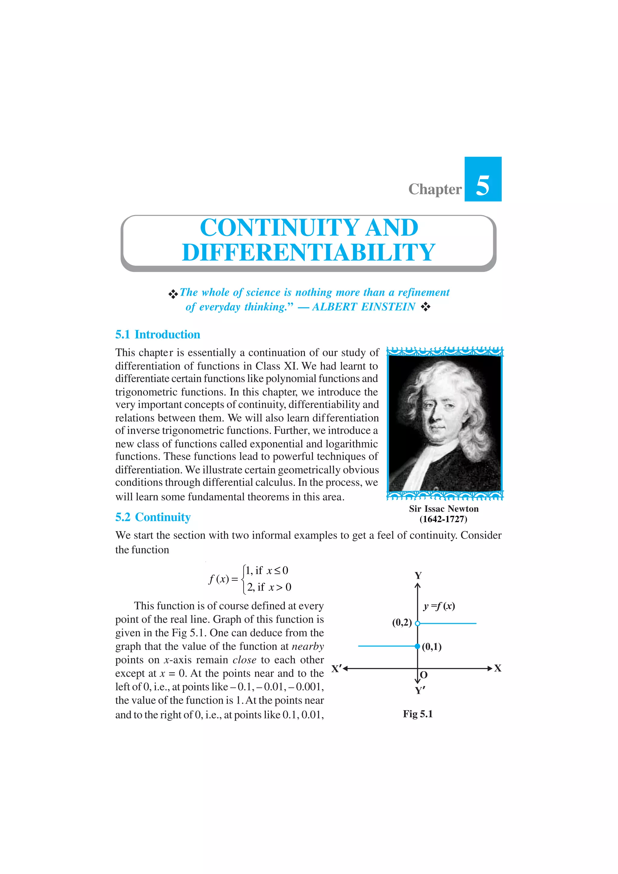
This document provides an introduction to the concepts of continuity and differentiability in calculus. It begins by giving two informal examples of functions that are and aren't continuous at a point to build intuition. It then provides a formal definition of continuity as the limit of a function at a point equaling the function value at that point. Several examples are worked through to demonstrate checking continuity at points and for entire functions. The document introduces the concept of limits approaching infinity to discuss the continuity of functions like 1/x. Overall, it lays the groundwork for understanding continuity and differentiability through examples and definitions.

1. The whole of science is nothing more than a refinement
of everyday thinking.” — ALBERT EINSTEIN
5.1 Introduction
This chapter is essentially a continuation of our study of
differentiation of functions in Class XI. We had learnt to
differentiate certain functions like polynomial functions and
trigonometric functions. In this chapter, we introduce the
very important concepts of continuity, differentiability and
relations between them. We will also learn differentiation
of inverse trigonometric functions. Further, we introduce a
new class of functions called exponential and logarithmic
functions. These functions lead to powerful techniques of
differentiation. We illustrate certain geometrically obvious
conditions through differential calculus. In the process, we
will learn some fundamental theorems in this area.
5.2 Continuity
We start the section with two informal examples to get a feel of continuity. Consider
the function
1, if 0
( )
2, if 0
x
f x
x
≤
= 
>
This function is of course defined at every
point of the real line. Graph of this function is
given in the Fig 5.1. One can deduce from the
graph that the value of the function at nearby
points on x-axis remain close to each other
except at x = 0. At the points near and to the
left of 0, i.e., at points like – 0.1, – 0.01, – 0.001,
the value of the function is 1.At the points near
and to the right of 0, i.e., at points like 0.1, 0.01,
Chapter 5
CONTINUITY AND
DIFFERENTIABILITY
Sir Issac Newton
(1642-1727)
Fig 5.1

2. MATHEMATICS148
0.001, the value of the function is 2. Using the language of left and right hand limits, we
may say that the left (respectively right) hand limit of f at 0 is 1 (respectively 2). In
particular the left and right hand limits do not coincide. We also observe that the value
of the function at x= 0 concides with the left hand limit. Note that when we try to draw
the graph, we cannot draw it in one stroke, i.e., without lifting pen from the plane of the
paper, we can not draw the graph of this function. In fact, we need to lift the pen when
we come to 0 from left. This is one instance of function being not continuous at x = 0.
Now, consider the function defined as
1,if 0
( )
2,if 0
x
f x
x
≠
= 
=
This function is also defined at every point. Left and the right hand limits at x = 0
are both equal to 1. But the value of the
function at x = 0 equals 2 which does not
coincide with the common value of the left
and right hand limits. Again, we note that we
cannot draw the graph of the function without
lifting the pen. This is yet another instance of
a function being not continuous at x = 0.
Naively, we may say that a function is
continuous at a fixed point if we can draw the
graph of the function aroundthat point without
lifting the pen from the plane of the paper.
Mathematically, it may be phrased precisely as follows:
Definition 1 Suppose f is a real function on a subset of the real numbers and let c be
a point in the domain of f. Then f is continuous at c if
lim ( ) ( )
x c
f x f c
→
=
More elaborately, if the left hand limit, right hand limit and the value of the function
at x = c exist and equal to each other, then f is said to be continuous at x =c. Recall that
if the right hand and left hand limits at x = c coincide, then we say that the common
value is the limit of the function at x= c. Hence we may also rephrase the definition of
continuity as follows: a function is continuous at x = c if the function is defined at
x = c and if the value of the function at x = c equals the limit of the function at
x = c. If f is not continuous at c, we say f is discontinuous at c and c is called a point
of discontinuity of f.
Fig 5.2

3. CONTINUITY AND DIFFERENTIABILITY 149
Example 1 Check the continuity of the function f given by f (x) = 2x + 3 at x = 1.
Solution First note that the function is defined at the given pointx = 1 and its value is 5.
Then find the limit of the function at x = 1. Clearly
1 1
lim ( ) lim(2 3) 2(1) 3 5
x x
f x x
→ →
= + = + =
Thus 1
lim ( ) 5 (1)
x
f x f
→
= =
Hence, f is continuous at x = 1.
Example 2 Examine whether the function f given by f (x) = x2
is continuous at x = 0.
Solution First note that the function is defined at the given pointx = 0 and its value is 0.
Then find the limit of the function at x = 0. Clearly
2 2
0 0
lim ( ) lim 0 0
x x
f x x
→ →
= = =
Thus 0
lim ( ) 0 (0)
x
f x f
→
= =
Hence, f is continuous at x = 0.
Example 3 Discuss the continuity of the function f given by f(x) = | x | at x = 0.
Solution By definition
f (x) =
,if 0
, if 0
x x
x x
− <

≥
Clearly the function is defined at 0 and f(0) = 0. Left hand limit of f at 0 is
0 0
lim ( ) lim (– ) 0
x x
f x x− −
→ →
= =
Similarly, the right hand limit of f at 0 is
0 0
lim ( ) lim 0
x x
f x x+ +
→ →
= =
Thus, the left hand limit, right hand limit and the value of the function coincide at
x = 0. Hence, f is continuous at x = 0.
Example 4 Show that the function f given by
f (x) =
3
3, if 0
1, if 0
x x
x
 + ≠

=
is not continuous at x = 0.

4. MATHEMATICS150
Solution The function is defined at x = 0 and its value at x = 0 is 1. When x ≠ 0, the
function is given by a polynomial. Hence,
0
lim ( )
x
f x
→
=
3 3
0
lim ( 3) 0 3 3
x
x
→
+ = + =
Since the limit of f atx = 0 does not coincide with f (0), the function is not continuous
at x = 0. It may be noted that x = 0 is the only point of discontinuity for this function.
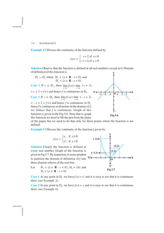
Example 5 Check the points where the constant function f (x) = k is continuous.
Solution The function is defined at all real numbers and by definition, its value at any
real number equals k. Let c be any real number. Then
lim ( )
x c
f x
→
= lim
x c
k k
→
=
Since f(c) = k = lim
x c→ f (x) for any real number c, the function f is continuous at
every real number.
Example 6 Prove that the identity function on real numbers given by f (x) = x is
continuous at every real number.
Solution The function is clearly defined at every point and f (c) = c for every real
number c.Also,
lim ( )
x c
f x
→
= lim
x c
x c
→
=
Thus, lim
x c→
f (x) = c = f(c) and hence the function is continuous at every real number.
Having defined continuity of a function at a given point, now we make a natural
extension of this definition to discuss continuity of a function.
Definition 2 Areal function f is said to be continuous if it is continuous at every point
in the domain of f.
This definition requires a bit of elaboration. Suppose f is a function defined on a
closed interval [a, b], then for f to be continuous, it needs to be continuous at every
point in [a, b] including the end points a and b. Continuity off at a means
lim ( )
x a
f x+
→
= f (a)
and continuity of f at b means
–
lim ( )
x b
f x
→
= f(b)
Observe that lim ( )
x a
f x−
→
and lim ( )
x b
f x+
→
do not make sense. As a consequence
of this definition, if f is defined only at one point, it is continuous there, i.e., if the
domain of f is a singleton, f is a continuous function.

5. CONTINUITY AND DIFFERENTIABILITY 151
Example 7 Is the function defined by f (x) = | x |, a continuous function?
Solution We may rewrite f as
f (x) =
,if 0
, if 0
x x
x x
− <

≥
By Example 3, we know that f is continuous at x = 0.
Let c be a real number such that c < 0. Then f (c) = – c. Also
lim ( )
x c
f x
→
= lim ( ) –
x c
x c
→
− = (Why?)
Since lim ( ) ( )
x c
f x f c
→
= , f is continuous at all negative real numbers.
Now, let c be a real number such that c > 0. Then f(c) = c. Also
lim ( )
x c
f x
→ = lim
x c
x c
→
= (Why?)
Since lim ( ) ( )
x c
f x f c
→
= , f is continuous at all positive real numbers. Hence, f
is continuous at all points.
Example 8 Discuss the continuity of the function f given by f (x) = x3
+ x2
– 1.
Solution Clearly f is defined at every real number c and its value at c is c3 + c2 – 1. We
also know that
lim ( )
x c
f x
→
=
3 2 3 2
lim ( 1) 1
x c
x x c c
→
+ − = + −
Thus lim ( ) ( )
x c
f x f c
→
= , and hence f is continuous at every real number.This means
f is a continuous function.
Example 9 Discuss the continuity of the function f defined by f (x) =
1
x
, x ≠ 0.
Solution Fix any non zero real number c, we have
1 1
lim ( ) lim
x c x c
f x
x c→ →
= =
Also, since forc ≠ 0,
1
( )f c
c
= , we have lim ( ) ( )
x c
f x f c
→
= and hence, f is continuous
at every point in the domain of f. Thus f is a continuous function.

6. MATHEMATICS152
We take this opportunity to explain the concept of infinity. This we do by analysing
the function f (x) =
1
x
near x = 0. To carry out this analysis we follow the usual trick of
finding the value of the function at real numbers close to 0. Essentially we are trying to
find the right hand limit of f at 0. We tabulate this in the following (Table 5.1).
Table 5.1
x 1 0.3 0.2 0.1 = 10–1 0.01 = 10–2 0.001 = 10–3 10–n
f (x) 1 3.333... 5 10 100 = 102
1000 = 103
10n
We observe that as x gets closer to 0 from the right, the value of f (x) shoots up
higher. This may be rephrased as: the value of f (x) may be made larger than any given
number by choosing a positive real number very close to 0. In symbols, we write
0
lim ( )
x
f x+
→
= + ∞
(to be read as: the right hand limit of f (x) at 0 is plus infinity). We wish to emphasise
that + ∞ is NOT a real number and hence the right hand limit of f at 0 does not exist (as
a real number).
Similarly, the left hand limit of f at 0 may be found. The following table is self
explanatory.
Table 5.2
x – 1 – 0.3 – 0.2 – 10–1
– 10–2
– 10–3
– 10–n
f (x) – 1 – 3.333... – 5 – 10 – 102 – 103 – 10n
From the Table 5.2, we deduce that the
value of f (x) may be made smaller than any
given number by choosing a negative real
number very close to 0. In symbols,
we write
0
lim ( )
x
f x−
→
= −∞
(to be read as: the left hand limit of f (x) at 0 is
minus infinity). Again, we wish to emphasise
that – ∞ is NOT a real number and hence the
left hand limit of f at 0 does not exist (as a real
number). The graph of the reciprocal function
given in Fig 5.3 is a geometric representation
of the above mentioned facts. Fig 5.3

7. CONTINUITY AND DIFFERENTIABILITY 153
Example 10 Discuss the continuity of the function f defined by
f (x) =
2, if 1
2,if 1
x x
x x
+ ≤

− >
Solution The function f is defined at all points of the real line.
Case 1 If c < 1, then f(c) = c + 2. Therefore, lim ( ) lim( 2) 2
x c x c
f x x c
→ →
= + = +
Thus,f is continuous at all real numbers less than 1.
Case 2 If c > 1, then f (c) = c – 2. Therefore,
lim ( ) lim
x c x c
f x
→ →
= (x – 2) = c – 2 = f (c)
Thus, f is continuous at all points x > 1.
Case 3 If c = 1, then the left hand limit of f at
x = 1 is
– –
1 1
lim ( ) lim ( 2) 1 2 3
x x
f x x
→ →
= + = + =
The right hand limit of f at x = 1 is
1 1
lim ( ) lim ( 2) 1 2 1
x x
f x x+ +
→ →
= − = − = −
Since the left and right hand limits of f at x = 1
do not coincide, f is not continuous at x = 1. Hence
x = 1 is the only point of discontinuity off. The graph of the function is given in Fig 5.4.
Example 11 Find all the points of discontinuity of the function f defined by
f (x) =
2, if 1
0, if 1
2,if 1
x x
x
x x
+ <

=
 − >
Solution As in the previous example we find that f
is continuous at all real numbers x ≠ 1. The left
hand limit of f at x = 1 is
–
1 1
lim ( ) lim ( 2) 1 2 3
x x
f x x−
→ →
= + = + =
The right hand limit of f at x = 1 is
1 1
lim ( ) lim ( 2) 1 2 1
x x
f x x+ +
→ →
= − = − = −
Since, the left and right hand limits of f at x = 1
do not coincide, f is not continuous atx = 1. Hence
x = 1 is the only point of discontinuity of f. The
graph of the function is given in the Fig 5.5.
Fig 5.4
Fig 5.5

8. MATHEMATICS154
Example 12 Discuss the continuity of the function defined by
f (x) =
2,if 0
2, if 0
x x
x x
+ <

− + >
Solution Observe that the function is defined at all real numbers except at 0. Domain
of definition of this function is
D1
∪ D2
where D1
= {x ∈ R : x < 0} and
D2
= {x ∈ R : x > 0}
Case 1 If c ∈ D1
, then lim ( ) lim
x c x c
f x
→ →
= (x + 2)
= c + 2 = f (c) and hence f is continuous in D1.
Case 2 If c ∈ D2, then lim ( ) lim
x c x c
f x
→ →
= (– x + 2)
= – c + 2 = f (c) and hence f is continuous in D2
.
Since f is continuous at all points in the domain of f,
we deduce that f is continuous. Graph of this
function is given in the Fig 5.6. Note that to graph
this function we need to lift the pen from the plane
of the paper, but we need to do that only for those points where the function is not
defined.
Example 13 Discuss the continuity of the function f given by
f (x) = 2
, if 0
, if 0
x x
x x
≥

<
Solution Clearly the function is defined at
every real number. Graph of the function is
given in Fig 5.7. By inspection, it seems prudent
to partition the domain of definition of f into
three disjoint subsets of the real line.
Let D1 = {x ∈ R : x < 0}, D2 = {0} and
D3 = {x ∈ R : x > 0}
Case 1 At any point in D1
, we have f (x) = x2
and it is easy to see that it is continuous
there (see Example 2).
Case 2 At any point in D3
, we have f (x) = x and it is easy to see that it is continuous
there (see Example 6).
Fig 5.6
Fig 5.7

9. CONTINUITY AND DIFFERENTIABILITY 155
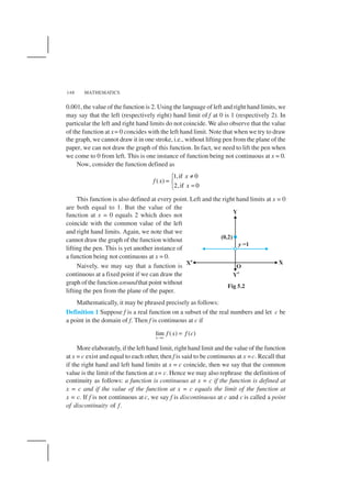
Case 3 Now we analyse the function at x= 0. The value of the function at 0 is f(0) = 0.
The left hand limit of f at 0 is
–
2 2
0 0
lim ( ) lim 0 0
x x
f x x−
→ →
= = =
The right hand limit of f at 0 is
0 0
lim ( ) lim 0
x x
f x x+ +
→ →
= =
Thus
0
lim ( ) 0
x
f x
→
= = f(0) and hence f is continuous at 0. This means that f is
continuous at every point in its domain and hence, f is a continuous function.
Example 14 Show that every polynomial function is continuous.
Solution Recall that a function p is a polynomial function if it is defined by
p(x) = a0
+ a1
x + ... + an
xn for some natural number n, an
≠ 0 and ai
∈ R. Clearly this
function is defined for every real number. For a fixed real number c, we have
lim ( ) ( )
x c
p x p c
→
=
By definition, p is continuous at c. Since c is any real number, p is continuous at
every real number and hence p is a continuous function.
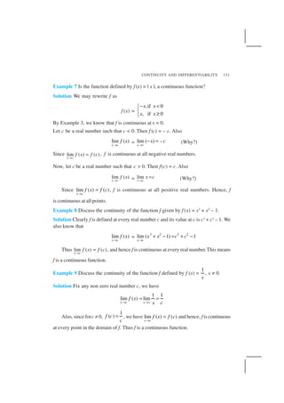
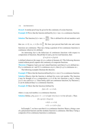
Example 15 Find all the points of discontinuity of the greatest integer function defined
by f (x) = [x], where [x] denotes the greatest integer less than or equal to x.
Solution First observe that f is defined for all real numbers. Graph of the function is
given in Fig 5.8. From the graph it looks like that f is discontinuous at every integral
point. Below we explore, if this is true.
Fig 5.8

10. MATHEMATICS156
Case 1 Letc be a real number which is not equal to any integer. It is evident from the
graph that for all real numbers close to c the value of the function is equal to [c]; i.e.,
lim ( ) lim [ ] [ ]
x c x c
f x x c
→ →
= = .Also f (c) = [c] and hence the function is continuous at all real
numbers not equal to integers.
Case 2 Let c be an integer. Then we can find a sufficiently small real number
r > 0 such that [c – r] = c – 1 whereas [c + r] = c.
This, in terms of limits mean that
lim
x c−
→
f (x) = c – 1, lim
x c+
→
f (x) = c
Since these limits cannot be equal to each other for any c, the function is
discontinuous at every integral point.
5.2.1 Algebra of continuous functions
In the previous class, after having understood the concept of limits, we learnt some
algebra of limits.Analogously, now we will study some algebra of continuous functions.
Since continuity of a function at a point is entirely dictated by the limit of the function at
that point, it is reasonable to expect results analogous to the case of limits.
Theorem 1 Suppose f and g be two real functions continuous at a real number c.
Then
(1) f + g is continuous at x = c.
(2) f – g is continuous at x = c.
(3) f . g is continuous at x = c.
(4)
f
g
 
 
 
is continuous at x = c, (provided g(c) ≠ 0).
Proof We are investigating continuity of (f + g) at x = c. Clearly it is defined at
x = c. We have
lim( )( )
x c
f g x
→
+ = lim[ ( ) ( )]
x c
f x g x
→
+ (by definition of f + g)
= lim ( ) lim ( )
x c x c
f x g x
→ →
+ (by the theorem on limits)
= f (c) + g(c) (as f and g are continuous)
= (f + g) (c) (by definition of f + g)
Hence, f + g is continuous at x = c.
Proofs for the remaining parts are similar and left as an exercise to the reader.

11. CONTINUITY AND DIFFERENTIABILITY 157
Remarks
(i) As a special case of (3) above, if f is a constant function, i.e., f (x) = λ for some
real number λ, then the function (λ . g) defined by (λ . g) (x) = λ . g(x) is also
continuous. In particular if λ = – 1, the continuity of f implies continuity of –f.
(ii) As a special case of (4) above, if f is the constant function f (x) = λ, then the
function
g
λ
defined by ( )
( )
x
g g x
λ λ
= is also continuous wherever g(x) ≠ 0. In
particular, the continuity of g implies continuity of
1
g
.
The above theorem can be exploited to generate many continuous functions. They
also aid in deciding if certain functions are continuous or not. The following examples
illustrate this:
Example 16 Prove that every rational function is continuous.
Solution Recall that every rational function f is given by
( )
( ) , ( ) 0
( )
p x
f x q x
q x
= ≠
where p and q are polynomial functions. The domain of f is all real numbers except
points at which qis zero. Since polynomial functions are continuous (Example 14), f is
continuous by (4) of Theorem 1.
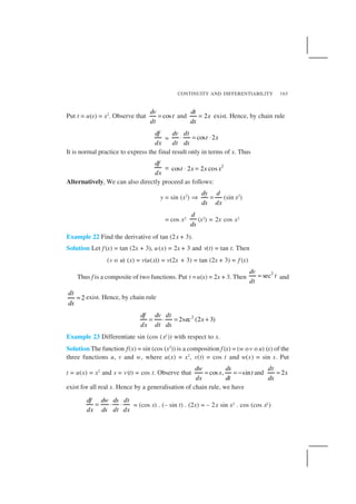
Example 17 Discuss the continuity of sine function.
Solution To see this we use the following facts
0
lim sin 0
x
x
→
=
We have not proved it, but is intuitively clear from the graph of sin x near 0.
Now, observe that f (x) = sin x is defined for every real number. Let c be a real
number. Put x = c + h. If x → c we know that h → 0. Therefore
lim ( )
x c
f x
→
= limsin
x c
x
→
= 0
lim sin( )
h
c h
→
+
= 0
lim[sin cos cos sin ]
h
c h c h
→
+
= 0 0
lim[sin cos ] lim [cos sin ]
h h
c h c h
→ →
+
= sin c + 0 = sin c = f (c)
Thus lim
x c→
f (x) = f (c) and hence f is a continuous function.

12. MATHEMATICS158
Remark Asimilar proof may be given for the continuity of cosine function.
Example 18 Prove that the function defined by f (x) = tan x is a continuous function.
Solution The function f (x) = tan x =
sin
cos
x
x
. This is defined for all real numbers such
that cos x ≠ 0, i.e., x ≠ (2n +1)
2
π
. We have just proved that both sine and cosine
functions are continuous. Thus tan x being a quotient of two continuous functions is
continuous wherever it is defined.
An interesting fact is the behaviour of continuous functions with respect to
composition of functions. Recall that if f and g are two real functions, then
(f o g) (x) = f (g(x))
is defined whenever the range of g is a subset of domain of f. The following theorem
(stated without proof) captures the continuity of composite functions.
Theorem 2 Suppose f and g are real valued functions such that (f o g) is defined at c.
If g is continuous at c and if f is continuous at g (c), then (f o g) is continuous at c.
The following examples illustrate this theorem.
Example 19 Show that the function defined by f(x) = sin (x2
) is a continuous function.
Solution Observe that the function is defined for every real number. The function
f may be thought of as a composition g o h of the two functions g and h, where
g(x) = sinx and h(x) = x2. Since bothg and h are continuous functions, by Theorem 2,
it can be deduced that f is a continuous function.
Example 20 Show that the function f defined by
f (x) = |1 – x + | x| |,
where x is any real number, is a continuous function.
Solution Define g by g(x) = 1 – x + | x| and h by h(x) = | x| for all real x. Then
(h o g) (x) = h(g (x))
= h(1– x + | x|)
= | 1– x + | x| | = f (x)
In Example 7, we have seen that h is a continuous function. Hence g being a sum
of a polynomial function and the modulus function is continuous. But then f being a
composite of two continuous functions is continuous.

13. CONTINUITY AND DIFFERENTIABILITY 159
EXERCISE 5.1
1. Prove that the function f(x) = 5x – 3 is continuous atx = 0, atx = – 3 and at x = 5.
2. Examine the continuity of the function f(x) = 2x2 – 1 at x = 3.
3. Examine the following functions for continuity.
(a) f (x) = x – 5 (b) f (x) =
1
5x −
, x ≠ 5
(c) f (x) =
2
25
5
x
x
−
+
, x ≠ –5 (d) f (x) = | x – 5|
4. Prove that the function f (x) = xn
is continuous at x = n, where n is a positive
integer.
5. Is the function f defined by
, if 1
( )
5, if > 1
x x
f x
x
≤
= 

continuous at x = 0? At x = 1? At x = 2?
Find all points of discontinuity of f, where f is defined by
6.
2 3, if 2
( )
2 3, if > 2
x x
f x
x x
+ ≤
= 
−
7.
| | 3, if 3
( ) 2 , if 3 < 3
6 2, if 3
x x
f x x x
x x
+ ≤ −

= − − <
 + ≥
8.
| |
, if 0
( )
0, if 0
x
x
f x x
x

≠
= 
 =
9.
, if 0
| |( )
1, if 0
x
x
xf x
x

<
= 
− ≥
10. 2
1, if 1
( )
1, if 1
x x
f x
x x
+ ≥
= 
+ <
11.
3
2
3, if 2
( )
1, if 2
x x
f x
x x
 − ≤
= 
+ >
12.
10
2
1, if 1
( )
, if 1
x x
f x
x x
 − ≤
= 
>
13. Is the function defined by
5, if 1
( )
5, if 1
x x
f x
x x
+ ≤
= 
− >
a continuous function?

14. MATHEMATICS160
Discuss the continuity of the function f, where f is defined by
14.
3, if 0 1
( ) 4, if 1 3
5, if 3 10
x
f x x
x
≤ ≤

= < <
 ≤ ≤
15.
2 , if 0
( ) 0, if 0 1
4 , if > 1
x x
f x x
x x
<

= ≤ ≤


16.
2, if 1
( ) 2 , if 1 1
2, if 1
x
f x x x
x
− ≤ −

= − < ≤
 >
17. Find the relationship between a and b so that the function f defined by
1, if 3
( )
3, if 3
ax x
f x
bx x
+ ≤
= 
+ >
is continuous at x = 3.
18. For what value of λ is the function defined by
2
( 2 ), if 0
( )
4 1, if 0
x x x
f x
x x
λ − ≤
= 
+ >
continuous at x = 0? What about continuity at x = 1?
19. Show that the function defined by g(x) = x – [x] is discontinuous at all integral
points. Here [x] denotes the greatest integer less than or equal to x.
20. Is the function defined by f(x) = x2
– sin x + 5 continuous at x = π?
21. Discuss the continuity of the following functions:
(a) f (x) = sin x + cos x (b) f (x) = sin x – cos x
(c) f (x) = sin x . cos x
22. Discuss the continuity of the cosine, cosecant, secant and cotangent functions.
23. Find all points of discontinuity of f, where
sin
, if 0
( )
1, if 0
x
x
f x x
x x

<
= 
 + ≥
24. Determine if f defined by
2 1
sin , if 0
( )
0, if 0
x x
f x x
x

≠
= 
 =
is a continuous function?

15. CONTINUITY AND DIFFERENTIABILITY 161
25. Examine the continuity of f, where f is defined by
sin cos , if 0
( )
1, if 0
x x x
f x
x
− ≠
= 
− =
Find the values of k so that the function f is continuous at the indicated point in Exercises
26 to 29.
26.
cos
, if
2 2
( )
3, if
2
k x
x
x
f x
x
π
≠π −
= 
π =

at x =
2
π
27.
2
, if 2
( )
3, if 2
kx x
f x
x
 ≤
= 
>
at x = 2
28.
1, if
( )
cos , if
kx x
f x
x x
+ ≤ π
= 
> π
at x = π
29.
1, if 5
( )
3 5, if 5
kx x
f x
x x
+ ≤
= 
− >
at x = 5
30. Find the values of a and b such that the function defined by
5, if 2
( ) , if 2 10
21, if 10
x
f x ax b x
x
≤

= + < <
 ≥
is a continuous function.
31. Show that the function defined by f (x) = cos (x2
) is a continuous function.
32. Show that the function defined by f(x) = | cos x | is a continuous function.
33. Examine that sin | x | is a continuous function.
34. Find all the points of discontinuity of f defined by f (x) = | x | – |x + 1|.
5.3. Differentiability
Recall the following facts from previous class. We had defined the derivative of a real
function as follows:
Suppose f is a real function and cis a point in its domain. The derivative of f at c is
defined by
0
( ) ( )
lim
h
f c h f c
h→
+ −

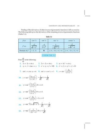
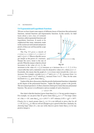
16. MATHEMATICS162
f (x) xn
sin x cos x tan x
f ′(x) nxn –1 cos x – sin x sec2 x
provided this limit exists. Derivative of f at c is denoted by f ′(c) or ( ( )) |c
d
f x
dx
. The
function defined by
0
( ) ( )
( ) lim
h
f x h f x
f x
h→
+ −
′ =
wherever the limit exists is defined to be the derivative of f. The derivative of f is
denoted by f ′(x) or ( ( ))
d
f x
dx
or if y = f (x) by
dy
dx
or y′. The process of finding
derivative of a function is called differentiation. We also use the phrase differentiate
f (x) with respect to x to mean find f ′(x).
The following rules were established as a part of algebra of derivatives:
(1) (u ± v)′ = u′ ± v′
(2) (uv)′ = u′v + uv′ (Leibnitz or product rule)
(3)
2
u u v uv
v v
′ ′ − ′ 
= 
 
, wherever v ≠ 0 (Quotient rule).
The following table gives a list of derivatives of certain standard functions:
Table 5.3
Whenever we defined derivative, we had put a caution provided the limit exists.
Now the natural question is; what if it doesn’t? The question is quite pertinent and so is
its answer. If
0
( ) ( )
lim
h
f c h f c
h→
+ −
does not exist, we say thatf is not differentiable at c.
In other words, we say that a function f is differentiable at a pointc in its domain if both
–
0
( ) ( )
lim
h
f c h f c
h→
+ −
and
0
( ) ( )
lim
h
f c h f c
h+
→
+ −
are finite and equal.Afunction is said
to be differentiable in an interval [a, b] if it is differentiable at every point of [a, b].As
in case of continuity, at the end pointsa and b, we take the right hand limit and left hand
limit, which are nothing but left hand derivative and right hand derivative of the function
at a and b respectively. Similarly, a function is said to be differentiable in an interval
(a, b) if it is differentiable at every point of (a, b).

17. CONTINUITY AND DIFFERENTIABILITY 163
Theorem 3 If a function f is differentiable at a point c, then it is also continuous at that
point.
Proof Since f is differentiable at c, we have
( ) ( )
lim ( )
x c
f x f c
f c
x c→
−
= ′
−
But for x ≠ c, we have
f (x) – f (c) =
( ) ( )
.( )
f x f c
x c
x c
−
−
−
Therefore lim[ ( ) ( )]
x c
f x f c
→
− =
( ) ( )
lim .( )
x c
f x f c
x c
x c→
− 
− − 
or lim[ ( )] lim[ ( )]
x c x c
f x f c
→ →
− =
( ) ( )
lim .lim[( )]
x c x c
f x f c
x c
x c→ →
− 
− − 
= f ′(c) . 0 = 0
or lim ( )
x c
f x
→
= f (c)
Hence f is continuous at x = c.
Corollary 1 Every differentiable function is continuous.
We remark that the converse of the above statement is not true. Indeed we have
seen that the function defined by f(x) = | x| is a continuous function. Consider the left
handlimit
–
0
(0 ) (0)
lim 1
h
f h f h
h h→
+ − −
= = −
The right hand limit
0
(0 ) (0)
lim 1
h
f h f h
h h+
→
+ −
= =
Since the above left and right hand limits at 0 are not equal, 0
(0 ) (0)
lim
h
f h f
h→
+ −
does not exist and hence f is not differentiable at 0. Thus f is not a differentiable
function.
5.3.1 Derivatives of composite functions
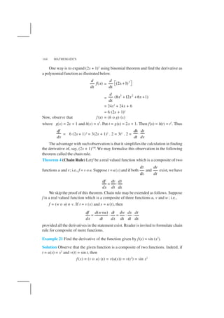
To study derivative of composite functions, we start with an illustrative example. Say,
we want to find the derivative of f, where
f (x) = (2x + 1)3

18. MATHEMATICS164
One way is to expand (2x + 1)3
using binomial theorem and find the derivative as
a polynomial function as illustrated below.
( )
d
f x
dx
=
3
(2 1)
d
x
dx
 + 
=
3 2
(8 12 6 1)
d
x x x
dx
+ + +
= 24x2
+ 24x + 6
= 6 (2x + 1)2
Now, observe that f (x) = (h o g) (x)
where g(x) = 2x + 1 and h(x) = x3
. Put t = g(x) = 2x + 1. Then f(x) = h(t) = t3
. Thus
df
dx
= 6 (2x + 1)2 = 3(2x + 1)2 . 2 = 3t2 . 2 =
dh dt
dt dx
⋅
The advantage with such observation is that it simplifies the calculation in finding
the derivative of, say, (2x + 1)100
. We may formalise this observation in the following
theorem called the chain rule.
Theorem 4 (Chain Rule) Letf be a real valued function which is a composite of two
functions u and v; i.e., f = v o u. Suppose t =u(x) and if both
dt
dx
and
dv
dt
exist,we have
df dv dt
dx dt dx
= ⋅
We skip the proof of this theorem. Chain rule may be extended as follows. Suppose
f is a real valued function which is a composite of three functions u, v and w ; i.e.,
f = (w o u) o v. If t = v (x) and s = u(t), then
( o )df d w u dt dw ds dt
dx dt dx ds dt dx
= ⋅ = ⋅ ⋅
provided all the derivatives in the statement exist. Reader is invited to formulate chain
rule for composite of more functions.
Example 21 Find the derivative of the function given by f (x) = sin (x2
).
Solution Observe that the given function is a composite of two functions. Indeed, if
t = u(x) = x2
and v(t) = sin t, then
f (x) = (v o u) (x) = v(u(x)) = v(x2
) = sin x2

19. CONTINUITY AND DIFFERENTIABILITY 165
Put t = u(x) = x2
. Observe that cos
dv
t
dt
= and 2
dt
x
dx
= exist. Hence, by chain rule
df
dx
= cos 2
dv dt
t x
dt dx
⋅ = ⋅
It is normal practice to express the final result only in terms of x. Thus
df
dx
= 2
cos 2 2 cost x x x⋅ =
Alternatively, We can also directly proceed as follows:
y = sin (x2
) ⇒
dy d
dx dx
= (sin x2
)
= cos x2
d
dx
(x2) = 2x cos x2
Example 22 Find the derivative of tan (2x + 3).
Solution Let f (x) = tan (2x + 3), u(x) = 2x + 3 and v(t) = tan t. Then
(v o u) (x) = v(u(x)) = v(2x + 3) = tan (2x + 3) = f (x)
Thus f is a composite of two functions. Put t =u(x) = 2x + 3. Then
2
sec
dv
t
dt
= and
2
dt
dx
= exist. Hence, by chain rule
2
2sec (2 3)
df dv dt
x
dx dt dx
= ⋅ = +
Example 23 Differentiate sin (cos (x2)) with respect to x.
Solution The function f(x) = sin (cos (x2
)) is a composition f (x) = (w ov o u) (x) of the
three functions u, v and w, where u(x) = x2
, v(t) = cos t and w(s) = sin s. Put
t = u(x) = x2
and s = v(t) = cos t. Observe that cos , sin
dw ds
s t
ds dt
= = − and 2
dt
x
dx
=
exist for all real x. Hence by a generalisation of chain rule, we have
df dw ds dt
dx ds dt dx
= ⋅ ⋅ = (cos s) . (– sin t) . (2x) = – 2x sin x2 . cos (cos x2)

20. MATHEMATICS166
Alternatively, we can proceed as follows:
y = sin (cos x2
)
Therefore
dy d
dx dx
= sin (cos x2
) = cos (cos x2
)
d
dx
(cos x2
)
= cos (cos x2
) (– sin x2
)
d
dx
(x2
)
= – sin x2
cos (cos x2
) (2x)
= – 2x sin x2
cos (cos x2
)
EXERCISE 5.2
Differentiate the functions with respect to x in Exercises 1 to 8.
1. sin (x2
+ 5) 2. cos (sin x) 3. sin (ax + b)
4. sec (tan ( x )) 5.
sin ( )
cos ( )
ax b
cx d
+
+ 6. cos x3
. sin2
(x5
)
7. ( )2
2 cot x 8. ( )cos x
9. Prove that the function f given by
f (x) = |x – 1|, x ∈ R
is not differentiable at x = 1.
10. Prove that the greatest integer function defined by
f (x) = [x], 0 < x < 3
is not differentiable at x = 1 and x = 2.
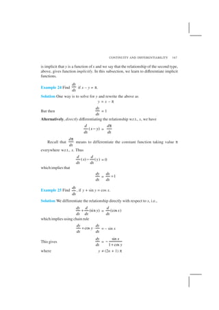
5.3.2 Derivatives of implicit functions
Until now we have been differentiating various functions given in the form y = f (x).
But it is not necessary that functions are always expressed in this form. For example,
consider one of the following relationships between x and y:
x – y – π = 0
x + sin xy – y = 0
In the first case, we can solve for y and rewrite the relationship as y = x – π. In
the second case, it does not seem that there is an easy way to solve for y. Nevertheless,
there is no doubt about the dependence of y on x in either of the cases. When a
relationship between x and y is expressed in a way that it is easy to solve for y and
write y = f (x), we say that y is given as an explicit function of x. In the latter case it

21. CONTINUITY AND DIFFERENTIABILITY 167
is implicit that y is a function ofx and we say that the relationship of the second type,
above, gives function implicitly. In this subsection, we learn to differentiate implicit
functions.
Example 24 Find
dy
dx
if x – y = π.
Solution One way is to solve for y and rewrite the above as
y = x – π
But then
dy
dx
= 1
Alternatively, directly differentiating the relationship w.r.t., x, we have
( )
d
x y
dx
− =
d
dx
π
Recall that
d
dx
π
means to differentiate the constant function taking value π
everywhere w.r.t., x. Thus
( ) ( )
d d
x y
dx dx
− = 0
which implies that
dy
dx
= 1
dx
dx
=
Example 25 Find
dy
dx
, if y + sin y = cos x.
Solution We differentiate the relationship directly with respect to x, i.e.,
(sin )
dy d
y
dx dx
+ = (cos )
d
x
dx
which implies using chain rule
cos
dy dy
y
dx dx
+ ⋅ = – sin x
This gives
dy
dx
=
sin
1 cos
x
y
−
+
where y ≠ (2n + 1) π

22. MATHEMATICS168
5.3.3 Derivatives of inverse trigonometric functions
We remark that inverse trigonometric functions are continuous functions, but we will
not prove this. Now we use chain rule to find derivatives of these functions.
Example 26 Find the derivative of f given by f (x) = sin–1
x assuming it exists.
Solution Let y = sin–1 x. Then, x = sin y.
Differentiating both sides w.r.t. x, we get
1 = cos y
dy
dx
which implies that
dy
dx
= 1
1 1
cos cos(sin )y x−
=
Observe that this is defined only for cos y ≠ 0, i.e., sin–1
x ≠ ,
2 2
π π
− , i.e.,x ≠ – 1, 1,
i.e., x ∈ (– 1, 1).
To make this result a bit more attractive, we carry out the following manipulation.
Recall that for x ∈ (– 1, 1), sin (sin–1 x) = x and hence
cos2
y = 1 – (sin y)2
= 1 – (sin (sin–1
x))2
= 1 – x2
Also, since y ∈ ,
2 2
π π 
− 
 
, cos y is positive and hence cos y = 2
1 x−
Thus, for x ∈ (– 1, 1),
2
1 1
cos 1
dy
dx y x
= =
−
Example 27 Find the derivative of f given by f (x) = tan–1 x assuming it exists.
Solution Let y = tan–1 x. Then, x = tan y.
Differentiating both sides w.r.t. x, we get
1 = sec2
y
dy
dx
which implies that
2 2 1 2 2
1 1 1 1
sec 1 tan 1 (tan(tan )) 1
dy
dx y y x x−
= = = =
+ + +

23. CONTINUITY AND DIFFERENTIABILITY 169
Finding of the derivatives of other inverse trigonometric functions is left as exercise.
The following table gives the derivatives of the remaining inverse trigonometric functions
(Table 5.4):
Table 5.4
f (x) cos–1
x cot–1
x sec–1
x cosec–1
x
f ′(x) 2
1
1 x
−
−
2
1
1 x
−
+ 2
1
1x x −
2
1
1x x
−
−
Domain of f ′ (–1, 1) R (–∞, –1) ∪ (1, ∞) (–∞, –1) ∪ (1, ∞)
EXERCISE 5.3
Find
dy
dx
in the following:
1. 2x + 3y = sin x 2. 2x + 3y = sin y 3. ax + by2
= cos y
4. xy + y2 = tan x + y 5. x2 + xy + y2 = 100 6. x3 + x2y + xy2 + y3 = 81
7. sin2 y + cos xy = κ 8. sin2 x + cos2 y = 1 9. y = sin–1
2
2
1
x
x
 
 
+ 
10. y = tan–1
3
2
3
,
1 3
x x
x
 −
 
− 
1 1
3 3
x− < <
11.
2
1
2
1 ,cos 0 1
1
x
y x
x
−  −
= < < 
+ 
12.
2
1
2
1 ,sin 0 1
1
x
y x
x
−  −
= < < 
+ 
13.
1
2
2 ,cos 1 1
1
x
y x
x
−  
= − < < 
+ 
14. ( )1 2 1 1,sin 2 1
2 2
y x x x−
= − − < <
15.
1
2
1 1
,sec 0
2 1 2
y x
x
−  
= < < 
− 

24. MATHEMATICS170
5.4 Exponential and Logarithmic Functions
Till now we have learnt some aspects of different classes of functions like polynomial
functions, rational functions and trigonometric functions. In this section, we shall
learn about a new class of (related)
functions called exponential functions and
logarithmic functions. It needs to be
emphasized that many statements made
in this section are motivational and precise
proofs of these are well beyond the scope
of this text.
The Fig 5.9 gives a sketch of
y = f1(x) = x, y = f2(x) = x2
, y = f3(x) = x3
and y = f4
(x) = x4
. Observe that the curves
get steeper as the power of x increases.
Steeper the curve, faster is the rate of
growth. What this means is that for a fixed
increment in the value of x (> 1), the
increment in the value of y = fn
(x) increases as n increases for n = 1, 2, 3, 4. It is
conceivable that such a statement is true for all positive values of n, where fn(x) = xn
.
Essentially, this means that the graph of y = fn (x) leans more towards the y-axis as n
increases. For example, consider f10(x) = x10
and f15 (x) = x15
. If x increases from 1 to
2, f10 increases from 1 to 210
whereas f15 increases from 1 to 215
. Thus, for the same
increment in x, f15
grow faster than f10
.
Upshotoftheabovediscussionisthatthegrowthofpolynomialfunctionsisdependent
on the degree of the polynomial function – higher the degree, greater is the growth.
The next natural question is: Is there a function which grows faster than any polynomial
function. The answer is in affirmative and an example of such a function is
y = f (x) = 10x.
Our claim is that this function f grows faster than fn(x) =xn
for any positive integer n.
For example, we can prove that 10x
grows faster than f100 (x) = x100
. For large values
of x like x = 103, note that f100
(x) = (103)100 = 10300 whereas f (103) = 3
10
10 = 101000.
Clearly f(x) is much greater than f100 (x). It is not difficult to prove that for all
x > 103
, f(x) > f100
(x). But we will not attempt to give a proof of this here. Similarly, by
choosing large values of x, one can verify that f(x) grows faster than fn
(x) for any
positive integer n.
Fig 5.9

25. CONTINUITY AND DIFFERENTIABILITY 171
Definition 3 The exponential function with positive base b > 1 is the function
y = f (x) = bx
The graph of y = 10x is given in the Fig 5.9.
It is advised that the reader plots this graph for particular values of b like 2, 3 and 4.
Following are some of the salient features of the exponential functions:
(1) Domain of the exponential function is R, the set of all real numbers.
(2) Range of the exponential function is the set of all positive real numbers.
(3) The point (0, 1) is always on the graph of the exponential function (this is a
restatement of the fact that b0
= 1 for any real b > 1).
(4) Exponential function is ever increasing; i.e., as we move from left to right, the
graph rises above.
(5) For very large negative values of x, the exponential function is very close to 0. In
other words, in the second quadrant, the graph approaches x-axis (but never
meets it).
Exponential function with base 10 is called the common exponential function. In
the Appendix A.1.4 of Class XI, it was observed that the sum of the series
1 1
1 ...
1! 2!
+ + +
is a number between 2 and 3 and is denoted by e. Using thise as the base we obtain an
extremely important exponential function y = ex.
This is called natural exponential function.
It would be interesting to know if the inverse of the exponential function exists and
has nice interpretation. This search motivates the following definition.
Definition 4 Let b > 1 be a real number. Then we say logarithm of a to base b is x if
bx = a.
Logarithm of a to base b is denoted by logb
a. Thus logb
a = x if bx = a. Let us
work with a few explicit examples to get a feel for this. We know 23
= 8. In terms of
logarithms, we may rewrite this as log2 8 = 3. Similarly, 104
= 10000 is equivalent to
saying log10 10000 = 4. Also, 625 = 54
= 252
is equivalent to saying log5 625 = 4 or
log25
625 = 2.
On a slightly more mature note, fixing a base b > 1, we may look at logarithm as
a function from positive real numbers to all real numbers. This function, called the
logarithmic function, is defined by
logb : R+
→ R
x → logb
x = y if by = x

26. MATHEMATICS172
As before if the base b = 10, we say it
is common logarithms and if b = e, then
we say it is natural logarithms. Often
natural logarithm is denoted by ln. In this
chapter, log x denotes the logarithm
function to base e, i.e., ln x will be written
assimplylog x.The Fig 5.10 gives the plots
of logarithm function to base 2, e and 10.
Some of the important observations
about the logarithm function to any base
b > 1 are listed below:
(1) We cannot make a meaningful definition of logarithm of non-positive numbers
and hence the domain of log function is R+.
(2) The range of log function is the set of all real numbers.
(3) The point (1, 0) is always on the graph of the log function.
(4) The log function is ever increasing,
i.e., as we move from left to right
the graph rises above.
(5) For x very near to zero, the value
of log x can be made lesser than
any given real number. In other
words in the fourth quadrant the
graph approaches y-axis (but never
meets it).
(6) Fig 5.11 gives the plot of y = ex and
y = ln x. It is of interest to observe
that the two curves are the mirror
images of each other reflected in the line y = x.
Two properties of ‘log’functions are proved below:
(1) There is a standard change of base rule to obtain loga
p in terms of logb
p. Let
loga
p = α, logb
p = β and logb
a = γ. This means aα
= p, bβ
= p and bγ
= a.
Substituting the third equation in the first one, we have
(bγ
)α
= bγα
= p
Using this in the second equation, we get
bβ = p = bγα
Fig 5.10
Fig 5.11

27. CONTINUITY AND DIFFERENTIABILITY 173
which implies β = αγ or α =
β
γ
. But then
loga
p =
log
log
b
b
p
a
(2) Another interesting property of the log function is its effect on products. Let
logb
pq = α. Then bα = pq. If logb
p = β and logb
q = γ, then bβ = p and bγ = q.
But then bα
= pq = bβ
bγ
= bβ + γ
which implies α = β + γ, i.e.,
logb
pq = logb
p + logb
q
A particularly interesting and important consequence of this is when p = q. In
this case the above may be rewritten as
logb
p2
= logb
p + logb
p = 2 log p
An easy generalisation of this (left as an exercise!) is
logb pn
= n log p
for any positive integer n. In fact this is true for any real number n, but we will
not attempt to prove this. On the similar lines the reader is invited to verify
logb
x
y
= logb
x – logb
y
Example 28 Is it true that x = elog x
for all real x?
Solution First, observe that the domain of log function is set of all positive real numbers.
So the above equation is not true for non-positive real numbers. Now, let y = elog x. If
y > 0, we may take logarithm which gives us logy = log (elog x
) = log x . log e = log x. Thus
y = x. Hence x = elog x
is true only for positive values of x.
One of the striking properties of the natural exponential function in differential
calculus is that it doesn’t change during the process of differentiation. This is captured
in the following theorem whose proof we skip.
Theorem 5*
(1) The derivative of ex w.r.t., x is ex; i.e.,
d
dx
(ex) = ex.
(2) The derivative of log x w.r.t., x is
1
x
; i.e.,
d
dx
(log x) =
1
x
.
* Please see supplementary material on Page 286.

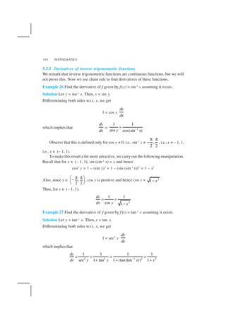
28. MATHEMATICS174
Example 29 Differentiate the following w.r.t. x:
(i) e–x
(ii) sin (log x), x > 0 (iii) cos–1
(ex
) (iv) ecos x
Solution
(i) Let y = e– x. Using chain rule, we have
dy
dx
=
x d
e
dx
−
⋅ (– x) = – e– x
(ii) Let y = sin (log x). Using chain rule, we have
dy
dx
=
cos (log )
cos (log ) (log )
d x
x x
dx x
⋅ =
(iii) Let y = cos–1 (ex). Using chain rule, we have
dy
dx
= 2 2
1
( )
1 ( ) 1
x
x
x x
d e
e
dxe e
− −
⋅ =
− −
(iv) Let y = ecos x
. Using chain rule, we have
dy
dx
= cos cos
( sin ) (sin )x x
e x x e⋅ − = −
EXERCISE 5.4
Differentiate the following w.r.t. x:
1.
sin
x
e
x
2.
1
sin x
e
−
3.
3
x
e
4. sin (tan–1 e–x) 5. log (cos ex) 6.
2 5
...x x x
e e e+ + +
7. , 0x
e x > 8. log (log x),x > 1 9.
cos
, 0
log
x
x
x
>
10. cos (log x + ex
), x > 0
5.5. Logarithmic Differentiation
In this section, we will learn to differentiate certain special class of functions given in
the form
y = f (x) = [u(x)]v (x)
By taking logarithm (to base e) the above may be rewritten as
logy = v(x) log [u(x)]

29. CONTINUITY AND DIFFERENTIABILITY 175
Using chain rule we may differentiate this to get
1 1
( )
( )
dy
v x
y dx u x
⋅ = ⋅ . u′(x) + v′(x) . log [u(x)]
which implies that
[ ]
( )
( ) ( ) log ( )
( )
dy v x
y u x v x u x
dx u x
 
= ⋅ ′ + ′ ⋅ 
 
The main point to be noted in this method is that f (x) and u(x) must always be
positive as otherwise their logarithms are not defined. This process of differentiation is
known as logarithms differentiation and is illustrated by the following examples:
Example 30 Differentiate
2
2
( 3)( 4)
3 4 5
x x
x x
− +
+ +
w.r.t. x.
Solution Let
2
2
( 3) ( 4)
(3 4 5)
x x
y
x x
− +
=
+ +
Taking logarithm on both sides, we have
log y =
1
2
[log (x – 3) + log (x2
+ 4) – log (3x2
+ 4x + 5)]
Now, differentiating both sides w.r.t. x, we get
1 dy
y dx
⋅ = 2 2
1 1 2 6 4
2 ( 3) 4 3 4 5
x x
x x x x
+ 
+ − − + + + 
or
dy
dx
= 2 2
1 2 6 4
2 ( 3) 4 3 4 5
y x x
x x x x
+ 
+ − − + + + 
=
2
2 2 2
1 ( 3)( 4) 1 2 6 4
2 ( 3)3 4 5 4 3 4 5
x x x x
xx x x x x
− + + 
+ − −+ + + + + 
Example 31 Differentiate ax
w.r.t. x, where a is a positive constant.
Solution Let y = ax
. Then
log y = x log a
Differentiating both sides w.r.t. x, we have
1 dy
y dx = log a

30. MATHEMATICS176
or
dy
dx
= y log a
Thus ( )xd
a
dx
= ax
log a
Alternatively ( )xd
a
dx
=
log log
( ) ( log )x a x ad d
e e x a
dx dx
=
= ex log a . log a = ax log a.
Example 32 Differentiate xsin x
, x > 0 w.r.t. x.
Solution Let y = xsin x
. Taking logarithm on both sides, we have
logy = sin x log x
Therefore
1
.
dy
y dx
= sin (log ) log (sin )
d d
x x x x
dx dx
+
or
1 dy
y dx =
1
(sin ) log cosx x x
x
+
or
dy
dx
=
sin
cos log
x
y x x
x
 
+  
=
sin sin
cos logx x
x x x
x
 
+  
= sin 1 sin
sin cos logx x
x x x x x−
⋅ + ⋅
Example 33 Find
dy
dx
, if yx
+ xy
+ xx
= ab
.
Solution Given that yx
+ xy
+ xx
= ab
.
Putting u = yx
, v = xy
and w = xx
, we get u + v + w = ab
Therefore 0
du dv dw
dx dx dx
+ + = ... (1)
Now, u = yx. Taking logarithm on both sides, we have
log u = x log y
Differentiating both sides w.r.t. x, we have

31. CONTINUITY AND DIFFERENTIABILITY 177
1 du
u dx
⋅ = (log ) log ( )
d d
x y y x
dx dx
+
=
1
log 1
dy
x y
y dx
⋅ + ⋅
So
du
dx
= log logxx dy x dy
u y y y
y dx y dx
   
+ = +   
   
... (2)
Also v = xy
Taking logarithm on both sides, we have
log v = y log x
Differentiating both sides w.r.t. x, we have
1 dv
v dx
⋅ = (log ) log
d dy
y x x
dx dx
+
=
1
log
dy
y x
x dx
⋅ + ⋅
So
dv
dx
= log
y dy
v x
x dx
 
+  
= logy y dy
x x
x dx
 
+  
... (3)
Again w = xx
Taking logarithm on both sides, we have
log w = x log x.
Differentiating both sides w.r.t. x, we have
1 dw
w dx
⋅ = (log ) log ( )
d d
x x x x
dx dx
+ ⋅
=
1
log 1x x
x
⋅ + ⋅
i.e.
dw
dx
= w (1 + log x)
= xx
(1 + log x) ... (4)

32. MATHEMATICS178
From (1), (2), (3), (4), we have
log logx yx dy y dy
y y x x
y dx x dx
   
+ + +     
+ xx (1 + log x) = 0
or (x . yx –1 + xy . log x)
dy
dx
= – xx (1 + log x) – y . xy–1 – yx log y
Therefore
dy
dx
=
1
1
[ log . (1 log )]
. log
x y x
x y
y y y x x x
x y x x
−
−
− + + +
+
EXERCISE 5.5
Differentiate the functions given in Exercises 1 to 11 w.r.t. x.
1. cos x . cos 2x . cos 3x 2.
( 1) ( 2)
( 3)( 4) ( 5)
x x
x x x
− −
− − −
3. (log x)cos x
4. xx
– 2sin x
5. (x + 3)2 . (x + 4)3 . (x + 5)4 6.
1
11
x
xx x
x
 + 
  
+ + 
 
7. (log x)x
+ xlog x
8. (sin x)x
+ sin–1
x
9. xsin x
+ (sin x)cos x
10.
2
cos
2
1
1
x x x
x
x
+
+
−
11. (x cos x)x
+
1
( sin )xx x
Find
dy
dx
of the functions given in Exercises 12 to 15.
12. xy + yx = 1 13. yx = xy
14. (cos x)y
= (cos y)x
15. xy = e(x – y)
16. Find the derivative of the function given by f(x) = (1 + x) (1 + x2
) (1 + x4
) (1 +x8
)
and hence find f ′(1).
17. Differentiate (x2 – 5x + 8) (x3 + 7x + 9) in three ways mentioned below:
(i) by using product rule
(ii) by expanding the product to obtain a single polynomial.
(iii) by logarithmic differentiation.
Do they all give the same answer?

33. CONTINUITY AND DIFFERENTIABILITY 179
18. If u, v and w are functions of x, then show that
d
dx
(u. v. w) =
du
dx
v. w + u .
dv
dx
. w + u . v
dw
dx
in two ways - first by repeated application of product rule, second by logarithmic
differentiation.
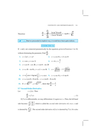
5.6 Derivatives of Functions in Parametric Forms
Sometimes the relation between two variables is neither explicit nor implicit, but some
link of a third variable with each of the two variables, separately, establishes a relation
between the first two variables. In such a situation, we say that the relation between
them is expressed via a third variable. The third variable is called the parameter. More
precisely, a relation expressed between two variables x and y in the form
x = f (t), y = g(t) is said to be parametric form with t as a parameter.
In order to find derivative of function in such form, we have by chain rule.
dy
dt
=
dy dx
dx dt
⋅
or
dy
dx
= whenever 0
dy
dxdt
dx dt
dt
 
≠ 
 
Thus
dy
dx
=
( )
as ( ) and ( )
( )
g t dy dx
g t f t
f t dt dt
′  
= ′ = ′ 
′  
[provided f ′(t) ≠ 0]
Example 34 Find
dy
dx
, if x = a cos θ, y = a sin θ.
Solution Given that
x = a cos θ, y = a sin θ
Therefore
dx
dθ
= – a sin θ,
dy
dθ
= a cos θ
Hence
dy
dx
=
cos
cot
sin
dy
ad
dx a
d
θθ = = − θ
− θ
θ

34. MATHEMATICS180
Example 35 Find
dy
dx
, if x = at2, y = 2at.
Solution Given that x = at2
, y = 2at
So
dx
dt
= 2at and
dy
dt
= 2a
Therefore
dy
dx
=
2 1
2
dy
adt
dx at t
dt
= =
Example 36 Find
dy
dx
, if x = a (θ + sin θ), y = a (1 – cos θ).
Solution We have
dx
dθ
= a(1 + cos θ),
dy
dθ
= a (sin θ)
Therefore
dy
dx
=
sin
tan
(1 cos ) 2
dy
ad
dx a
d
θ θθ = =
+ θ
θ
Note It may be noted here that
dy
dx
is expressed in terms of parameter only
without directly involving the main variables x and y.
Example 37 Find
2 2 2
3 3 3, if
dy
x y a
dx
+ = .
Solution Let x = a cos3 θ, y = a sin3 θ. Then
2 2
3 3x y+ =
2 2
3 33 3
( cos ) ( sin )a aθ + θ
=
2 2
2 23 3(cos (sin )a aθ + θ =
Hence, x = a cos3
θ, y = a sin3
θ is parametric equation of
2 2 2
3 3 3x y a+ =
Now
dx
dθ
= – 3a cos2
θ sin θ and
dy
dθ
= 3a sin2
θ cos θ

35. CONTINUITY AND DIFFERENTIABILITY 181
Therefore
dy
dx
=
2
3
2
3 sin cos
tan
3 cos sin
dy
a yd
dx xa
d
θ θθ = = − θ = −
− θ θ
θ
Note Had we proceeded in implicit way, it would have been quite tedious.
EXERCISE 5.6
If x and y are connected parametrically by the equations given in Exercises 1 to 10,
without eliminating the parameter, Find
dy
dx
.
1. x = 2at2, y = at4 2. x = a cos θ, y = b cos θ
3. x = sin t, y = cos 2t 4. x = 4t, y =
4
t
5. x = cos θ – cos 2θ, y = sin θ – sin 2θ
6. x = a (θ – sin θ), y = a (1 + cos θ) 7. x =
3
sin
cos 2
t
t
,
3
cos
cos2
t
y
t
=
8. cos log tan
2
t
x a t
 
= + 
 
y = a sin t 9. x = a sec θ, y = b tan θ
10. x = a (cos θ + θ sin θ), y = a (sin θ – θ cos θ)
11. If
1 1
sin cos
, , show thatt t dy y
x a y a
dx x
− −
= = = −
5.7 Second Order Derivative
Let y = f (x). Then
dy
dx
= f ′(x) ... (1)
If f′(x) is differentiable, we may differentiate (1) again w.r.t. x.Then, the left hand
side becomes
d dy
dx dx
 
 
 
which is called the second order derivative of y w.r.t. x and
is denoted by
2
2
d y
dx
. The second order derivative off (x) is denoted by f ″(x). It is also

36. MATHEMATICS182
denoted by D2
y or y″ or y2 ify = f (x). We remark that higher order derivatives may be
defined similarly.
Example 38 Find
2
2
d y
dx
, if y = x3
+ tan x.
Solution Given that y = x3
+ tan x. Then
dy
dx
= 3x2
+ sec2
x
Therefore
2
2
d y
dx
= ( )2 2
3 sec
d
x x
dx
+
= 6x + 2 sec x . sec x tan x = 6x + 2 sec2 x tan x
Example 39 If y = A sin x + B cos x, then prove that
2
2
0
d y
y
dx
+ = .
Solution We have
dy
dx
= A cos x – B sin x
and
2
2
d y
dx
=
d
dx
(A cos x – B sin x)
= – A sin x – B cos x = – y
Hence
2
2
d y
dx
+ y = 0
Example 40 If y = 3e2x + 2e3x, prove that
2
2
5 6 0
d y dy
y
dxdx
− + = .
Solution Given that y = 3e2x + 2e3x. Then
dy
dx
= 6e2x + 6e3x = 6 (e2x + e3x)
Therefore
2
2
d y
dx
= 12e2x
+ 18e3x
= 6 (2e2x
+ 3e3x
)
Hence
2
2
5
d y dy
dxdx
− + 6y = 6 (2e2x
+ 3e3x
)
– 30 (e2x + e3x) + 6 (3e2x + 2e3x) = 0

37. CONTINUITY AND DIFFERENTIABILITY 183
Example 41 If y = sin–1
x, show that (1 – x2
)
2
2
0
d y dy
x
dxdx
− = .
Solution We have y = sin–1
x. Then
dy
dx
= 2
1
(1 )x−
or
2
(1 ) 1
dy
x
dx
− =
So
2
(1 ) . 0
d dy
x
dx dx
 
− = 
 
or ( )
2
2 2
2
(1 ) (1 ) 0
d y dy d
x x
dx dxdx
− ⋅ + ⋅ − =
or
2
2
2 2
2
(1 ) 0
2 1
d y dy x
x
dxdx x
− ⋅ − ⋅ =
−
Hence
2
2
2
(1 ) 0
d y dy
x x
dxdx
− − =
Alternatively, Given that y = sin–1 x, we have
1
2
1
1
y
x
=
−
, i.e., ( )2 2
1
1 1x y− =
So 2 2
1 2 1(1 ). 2 (0 2 ) 0x y y y x− + − =
Hence (1 – x2) y2
– xy1
= 0
EXERCISE 5.7
Find the second order derivatives of the functions given in Exercises 1 to 10.
1. x2
+ 3x + 2 2. x20
3. x . cos x
4. log x 5. x3
log x 6. ex
sin 5x
7. e6x
cos 3x 8. tan–1
x 9. log (log x)
10. sin (log x)
11. If y = 5 cos x – 3 sin x, prove that
2
2
0
d y
y
dx
+ =

38. MATHEMATICS184
12. If y = cos–1 x, Find
2
2
d y
dx
in terms of y alone.
13. If y = 3 cos (log x) + 4 sin (log x), show that x2
y2 + xy1 + y = 0
14. If y = Aemx
+ Benx
, show that
2
2
( ) 0
d y dy
m n mny
dxdx
− + + =
15. If y = 500e7x
+ 600e–7x
, show that
2
2
49
d y
y
dx
=
16. If ey
(x + 1) = 1, show that
22
2
d y dy
dxdx
 
=  
 
17. If y = (tan–1
x)2
, show that (x2
+ 1)2
y2
+ 2x (x2
+ 1) y1
= 2
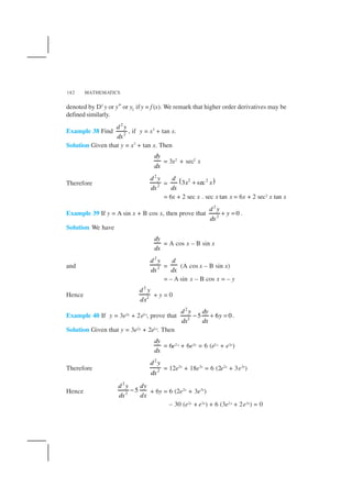
5.8 Mean Value Theorem
In this section, we will state two fundamental results in Calculus without proof. We
shall also learn the geometric interpretation of these theorems.
Theorem 6 (Rolle’s Theorem) Let f : [a, b] → R be continuous on [a, b] and
differentiable on (a, b), such that f(a) = f(b), where a and b are some real numbers.
Then there exists some c in (a, b) such that f ′(c) = 0.
In Fig 5.12 and 5.13, graphs of a few typical differentiable functions satisfying the
hypothesis of Rolle’s theorem are given.
Fig 5.12 Fig 5.13
Observe what happens to the slope of the tangent to the curve at various points
between a and b. In each of the graphs, the slope becomes zero at least at one point.
That is precisely the claim of the Rolle’s theorem as the slope of the tangent at any
point on the graph of y = f (x) is nothing but the derivative of f (x) at that point.

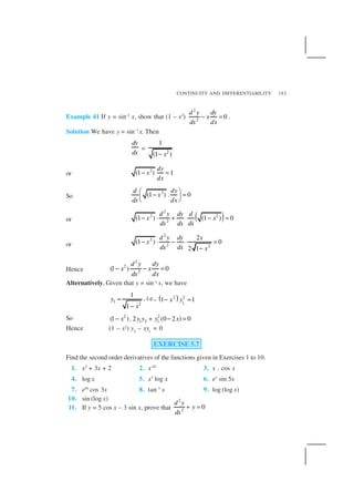
39. CONTINUITY AND DIFFERENTIABILITY 185
Theorem 7 (Mean Value Theorem) Let f : [a, b] → R be a continuous function on
[a, b] and differentiable on (a, b). Then there exists some c in (a, b) such that
( ) ( )
( )
f b f a
f c
b a
−
′ =
−
Observe that the Mean Value Theorem (MVT) is an extension of Rolle’s theorem.
Let us now understand a geometric interpretation of the MVT.The graph of a function
y = f(x) is given in the Fig 5.14. We have already interpreted f′(c) as the slope of the
tangent to the curve y = f (x) at (c, f (c)). From the Fig 5.14 it is clear that
( ) ( )f b f a
b a
−
−
is the slope of the secant drawn between (a, f (a)) and (b, f(b)). The MVT states that
there is a point c in (a, b) such that the slope of the tangent at (c, f(c)) is same as the
slope of the secant between (a, f (a)) and (b, f(b)). In other words, there is a point c in
(a, b) such that the tangent at (c, f(c)) is parallel to the secant between (a, f(a)) and
(b, f (b)).
Fig 5.14
Example 42 Verify Rolle’s theorem for the function y = x2 + 2, a = – 2 and b = 2.
Solution The function y = x2 + 2 is continuous in [– 2, 2] and differentiable in (– 2, 2).
Also f(– 2) = f( 2) = 6 and hence the value of f(x) at – 2 and 2 coincide. Rolle’s
theorem states that there is a point c ∈ (– 2, 2), where f′(c) = 0. Since f′(x) = 2x, we
get c = 0. Thus at c = 0, we have f′(c) = 0 and c = 0 ∈ (– 2, 2).
Example 43Verify MeanValue Theorem for the functionf (x) = x2 in the interval [2, 4].
Solution The function f(x) = x2 is continuous in [2, 4] and differentiable in (2, 4) as its
derivative f′(x) = 2x is defined in (2, 4).

40. MATHEMATICS186
Now, f(2) = 4 and f (4) = 16. Hence
( ) ( ) 16 4
6
4 2
f b f a
b a
− −
= =
− −
MVT states that there is a point c ∈ (2, 4) such that f′(c) = 6. But f′(x) = 2x which
implies c = 3. Thus at c = 3 ∈ (2, 4), we have f′(c) = 6.
EXERCISE 5.8
1. Verify Rolle’s theorem for the function f (x) = x2
+ 2x – 8, x ∈ [– 4, 2].
2. Examine if Rolle’s theorem is applicable to any of the following functions. Can
you say some thing about the converse of Rolle’s theorem from these example?
(i) f(x) = [x] for x ∈ [5, 9] (ii) f(x) = [x] for x ∈ [– 2, 2]
(iii) f(x) = x2
– 1 for x ∈ [1, 2]
3. If f : [– 5, 5] → R is a differentiable function and if f ′(x) does not vanish
anywhere, then prove that f(– 5) ≠ f(5).
4. Verify Mean Value Theorem, if f (x) = x2 – 4x – 3 in the interval [a, b], where
a = 1 and b = 4.
5. Verify Mean Value Theorem, if f(x) = x3
– 5x2
– 3x in the interval [a, b], where
a = 1 and b = 3. Find all c ∈ (1, 3) for which f′(c) = 0.
6. Examine the applicability of MeanValue Theorem for all three functions given in
the above exercise 2.
Miscellaneous Examples
Example 44 Differentiate w.r.t. x, the following function:
(i)
2
1
3 2
2 4
x
x
+ +
+
(ii)
2
sec –1
3cosx
e x+ (iii) log7
(log x)
Solution
(i) Let y = 2
1
3 2
2 4
x
x
+ +
+
=
1 1
22 2(3 2) (2 4)x x
−
+ + +
Note that this function is defined at all real numbers
2
3
x > − . Therefore
dy
dx
=
1 1
1 1
2 22 2
1 1
(3 2) (3 2) (2 4) (2 4)
2 2
d d
x x x x
dx dx
− − − 
+ ⋅ + + − + ⋅ + 
 

41. CONTINUITY AND DIFFERENTIABILITY 187
=
1 3
22 2
1 1
(3 2) (3) (2 4) 4
2 2
x x x
− − 
+ ⋅ − + ⋅  
=
( )
3
2 2
3 2
2 3 2
2 4
x
x
x
−
+
+
This is defined for all real numbers
2
3
x > − .
(ii) Let
2
sec 1
3cosx
y e x−
= +
This is defined at every real number in [ 1,1]− . Therefore
dy
dx
=
2
sec 2
2
1
(sec ) 3
1
x d
e x
dx x
 
⋅ + −  −
=
2
sec
2
1
2sec (sec ) 3
1
x d
e x x
dx x
   
⋅ + −      −
=
2
sec
2
1
2sec (sec tan ) 3
1
x
x x x e
x
 
+ − 
− 
=
2
2 sec
2
1
2sec tan 3
1
x
x x e
x
 
+ − 
− 
Observe that the derivative of the given function is valid only in { }[ 1,1] 0− − as
the derivative of cos–1
x exists only in (– 1, 1) and the function itself is not
defined at 0.
(iii) Let y = log7
(log x) =
log (log )
log7
x
(by change of base formula).
The function is defined for all real numbers x > 1. Therefore
dy
dx
=
1
(log (log ))
log7
d
x
dx
=
1 1
(log )
log7 log
d
x
x dx
⋅
=
1
log7logx x

42. MATHEMATICS188
Example 45 Differentiate the following w.r.t. x.
(i) cos –1
(sin x) (ii) 1 sin
tan
1 cos
x
x
−  
 
+ 
(iii)
1
1 2
sin
1 4
x
x
+
−  
 
+ 
Solution
(i) Let f (x) = cos –1 (sin x). Observe that this function is defined for all real numbers.
We may rewrite this function as
f(x) = cos –1
(sin x)
=
1
cos cos
2
x−  π 
−    
=
2
x
π
−
Thus f ′(x) = – 1.
(ii) Let f (x) = tan–1 sin
1 cos
x
x
 
 
+ 
. Observe that this function is defined for all real
numbers, where cos x ≠ – 1; i.e., at all odd multiplies of π. We may rewrite this
function as
f(x) =
1 sin
tan
1 cos
x
x
−  
 
+ 
=
1
2
2 sin cos
2 2tan
2cos
2
x x
x
−
    
       
 
 
  
=
1
tan tan
2 2
x x−   
=    
Observe that we could cancel cos
2
x 
 
 
in both numerator and denominator as it
is not equal to zero. Thus f′(x) =
1.
2
(iii) Let f(x) = sin–1
1
2
1 4
x
x
+
 
 
+ 
.To find the domain of this function we need to find all
x such that
1
2
1 1
1 4
x
x
+
− ≤ ≤
+
. Since the quantity in the middle is always positive,

43. CONTINUITY AND DIFFERENTIABILITY 189
we need to find all x such that
1
2
1
1 4
x
x
+
≤
+
, i.e., all x such that 2x + 1
≤ 1 + 4x
. We
may rewrite this as 2 ≤
1
2x + 2x
which is true for all x. Hence the function
is defined at every real number. By putting 2x
= tan θ, this function may be
rewritten as
f(x) =
1
1 2
sin
1 4
x
x
+
−  
 
+ 
=
( )
1
2
2 2
sin
1 2
x
x
−  ⋅
 
 + 
=
1
2
2tan
sin
1 tan
− θ 
 + θ 
= sin–1
[sin 2θ]
= 2θ = 2 tan–1 (2x)
Thus f ′(x) =
( )2
1
2 (2 )
1 2
x
x
d
dx
⋅ ⋅
+
=
2
(2 )log 2
1 4
x
x
⋅
+
=
1
2 log2
1 4
x
x
+
+
Example 46 Find f ′(x) if f(x) = (sin x)sin x for all 0 < x < π.
Solution The function y = (sin x)sin x
is defined for all positive real numbers. Taking
logarithms, we have
log y = log (sin x)sin x
= sin x log (sin x)
Then
1 dy
y dx
=
d
dx
(sin x log (sin x))
= cos x log (sin x) + sin x .
1
(sin )
sin
d
x
x dx
⋅
= cos x log (sin x) + cos x
= (1 + log (sin x)) cos x

44. MATHEMATICS190
Thus
dy
dx
= y((1 + log (sin x)) cos x) = (1 + log (sin x)) ( sin x)sin x cos x
Example 47 For a positive constant a find
dy
dx
, where
1
1
, and
a
t
ty a x t
t
+  
= = + 
 
Solution Observe that both y and x are defined for all real t ≠ 0. Clearly
dy
dt
= ( )1
t
t
d
adt
+
=
1
1
log
t
t
d
a t a
dt t
+  
+ ⋅ 
 
=
1
2
1
1 log
t
ta a
t
+  
− 
 
Similarly
dx
dt
=
1
1 1
a
d
a t t
t dt t
−
   
+ ⋅ +     
=
1
2
1 1
1
a
a t
t t
−
   
+ ⋅ −     
dx
dt
≠ 0 only if t ≠ ± 1. Thus for t ≠ ± 1,
dy
dy dt
dxdx
dt
= =
1
2
1
2
1
1 log
1 1
1
t
t
a
a a
t
a t
t t
+
−
 
−  
   
+ ⋅ −     
=
1
1
log
1
t
t
a
a a
a t
t
+
−
 
+ 
 
Example 48 Differentiate sin2 x w.r.t. ecos x.
Solution Let u (x) = sin2
x and v (x) = ecos x
. We want to find /
/
du du dx
dv dv dx
= . Clearly
du
dx
= 2 sin x cos x and
dv
dx
= ecos x (– sin x) = – (sin x) ecos x

45. CONTINUITY AND DIFFERENTIABILITY 191
Thus
du
dv
= cos cos
2sin cos 2cos
sin x x
x x x
x e e
= −
−
Miscellaneous Exercise on Chapter 5
Differentiate w.r.t. x the function in Exercises 1 to 11.
1. (3x2 – 9x + 5)9 2. sin3 x + cos6 x
3. (5x)3 cos 2x
4. sin–1
(x x ), 0 ≤ x ≤ 1
5.
1
cos
2
2 7
x
x
−
+
, – 2 < x < 2
6.
1 1 sin 1 sin
cot
1 sin 1 sin
x x
x x
−
 + + −
 
+ − − 
, 0 < x <
2
π
7. (log x)log x, x > 1
8. cos (a cos x + b sin x), for some constant a and b.
9. (sin x – cos x) (sin x – cos x)
,
3
4 4
x
π π
< <
10. xx + xa + ax + aa, for some fixed a > 0 and x > 0
11. ( )
22
3
3
xx
x x−
+ − , for x > 3
12. Find
dy
dx
, if y = 12 (1 – cos t), x = 10 (t – sin t),
2 2
t
π π
− < <
13. Find
dy
dx
, if y = sin–1
x + sin–1 2
1 x− , 0 < x < 1
14. If 1 1 0x y y x+ + + = , for , – 1 < x < 1, prove that
( )2
1
1
dy
dx x
= −
+
15. If (x – a)2
+ (y – b)2
= c2
, for some c > 0, prove that
3
2 2
2
2
1
dy
dx
d y
dx
  +  
  
is a constant independent of a and b.

46. MATHEMATICS192
16. If cos y = x cos (a + y), with cos a ≠ ± 1, prove that
2
cos ( )
sin
dy a y
dx a
+
= .
17. If x = a (cos t + t sin t) and y = a (sin t – t cos t), find
2
2
d y
dx
.
18. If f (x) = | x |3
, show that f ″(x) exists for all real x and find it.
19. Using mathematical induction prove that ( ) 1n nd
x nx
dx
−
= for all positive
integers n.
20. Using the fact that sin (A + B) = sin Acos B + cos Asin B and the differentiation,
obtain the sum formula for cosines.
21. Does there exist a function which is continuous everywhere but not differentiable
at exactly two points? Justify your answer.
22. If
( ) ( ) ( )f x g x h x
y l m n
a b c
= , prove that
( ) ( ) ( )f x g x h x
dy
l m n
dx
a b c
′ ′ ′
=
23. If y = 1
cosa x
e
−
, – 1 ≤ x ≤ 1, show that ( )
2
2 2
2
1 0
d y dy
x x a y
dxdx
− − − = .
Summary
A real valued function is continuous at a point in its domain if the limit of the
function at that point equals the value of the function at that point.Afunction
is continuous if it is continuous on the whole of its domain.
Sum, difference, product and quotient of continuous functions are continuous.
i.e., if f and g are continuous functions, then
(f ± g) (x) = f (x) ± g(x) is continuous.
(f . g) (x) = f (x) . g(x) is continuous.
( )
( )
( )
f f x
x
g g x
 
= 
 
(wherever g(x) ≠ 0) is continuous.
Every differentiable function is continuous, but the converse is not true.

47. CONTINUITY AND DIFFERENTIABILITY 193
Chain rule is rule to differentiate composites of functions. Iff = v o u, t =u (x)
and if both
dt
dx
and
dv
dt
exist then
df dv dt
dx dt dx
= ⋅
Following are some of the standard derivatives (in appropriate domains):
( )1
2
1
sin
1
d
x
dx x
−
=
−
( )1
2
1
cos
1
d
x
dx x
−
= −
−
( )1
2
1
tan
1
d
x
dx x
−
=
+
( )1
2
1
cot
1
d
x
dx x
− −
=
+
( )1
2
1
sec
1
d
x
dx x x
−
=
−
( )1
2
1
cosec
1
d
x
dx x x
− −
=
−
( )x xd
e e
dx
= ( )
1
log
d
x
dx x
=
Logarithmic differentiation is a powerful technique to differentiate functions
of the form f (x) = [u (x)]v (x). Here both f(x) and u(x) need to be positive for
this technique to make sense.
Rolle’s Theorem: If f : [a, b] → R is continuous on [a, b] and differentiable
on (a, b) such that f (a) = f (b), then there exists some c in (a, b) such that
f ′(c) = 0.
Mean Value Theorem: If f : [a, b] → R is continuous on [a, b] and
differentiable on (a, b). Then there exists some c in (a, b) such that
( ) ( )
( )
f b f a
f c
b a
−
′ =
−
— —