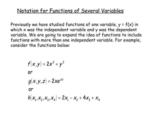
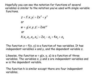
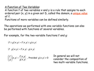
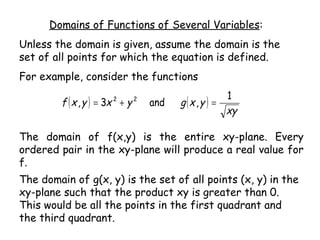
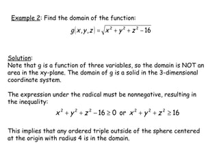
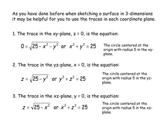
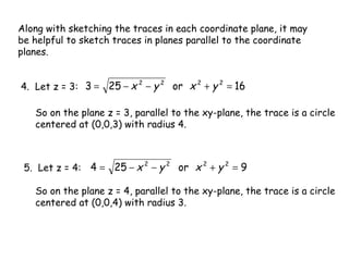
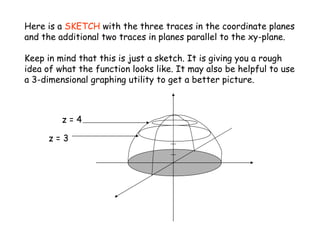
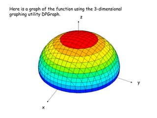
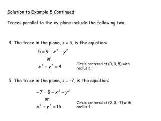
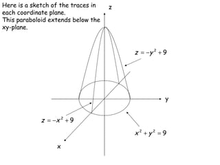
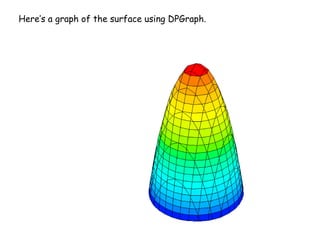
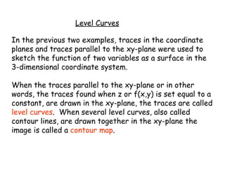
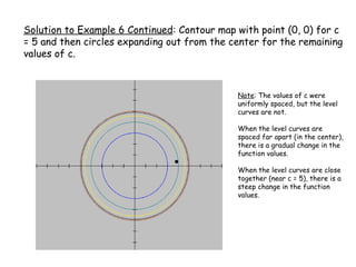
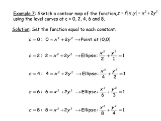
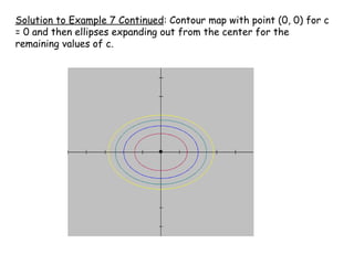
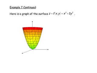
SlideShare a Scribd company logo
Chapter 8: Functions of Several Variables Section 8.1 Introduction to Functions of Several Variables Written by Karen Overman Instructor of Mathematics Tidewater Community College, Virginia Beach Campus  Virginia Beach, VA With Assistance from a VCCS LearningWare Grant
[object Object],[object Object],[object Object],[object Object],[object Object]
Notation for Functions of Several Variables Previously we have studied functions of one variable, y = f(x) in which x was the independent variable and y was the dependent variable. We are going to expand the idea of functions to include functions with more than one independent variable. For example, consider the functions below:
The function z = f(x, y) is a function of two variables. It has independent variables x and y, and the dependent variable z.  Likewise, the function w = g(x, y, z) is a function of three variables. The variables x, y and z are independent variables and w is the dependent variable.  The function h is similar except there are four independent variables. Hopefully you can see the notation for functions of several variables is similar to the notation you’ve used with single variable  functions.
When finding values of the several variable functions instead of just substituting in an x-value, we will substitute in values for each of the independent variables: For example, using the function f on the previous slide, we will  evaluate the function f(x, y) for (2, 3) , (4, -3) and (5, y).
A Function of Two Variables :  A function f of two variables x and y is a rule that assigns to each ordered pair (x, y) in a given set D, called the domain, a  unique value  of f. Functions of more variables can be defined similarly. The operations we performed with one-variable functions can also be performed with functions of several variables.  For example, for the two-variable functions f and g: In general we will not consider the composition of two multi-variable functions.
Domains of Functions of Several Variables : Unless the domain is given, assume the domain is the set of all points for which the equation is defined.  For example, consider the functions  The domain of f(x,y) is the entire xy-plane. Every ordered pair in the xy-plane will produce a real value for f. The domain of g(x, y) is the set of all points (x, y) in the xy-plane such that the product xy is greater than 0. This would be all the points in the first quadrant and the third quadrant.
Example 1 : Find the domain of the function: Solution : The domain of f(x, y) is the set of all points that satisfy the inequality:  or You may recognize that this is similar to the equation of a circle and the inequality implies that any ordered pair on the circle or inside  the circle  is in the domain.  x y The highlighted area is the domain to f.
Example 2 : Find the domain of the function: Solution :  Note that g is a function of three variables, so the domain is NOT an area in the xy-plane. The domain of g is a solid in the 3-dimensional coordinate system.  The expression under the radical must be nonnegative, resulting in the inequality: This implies that any ordered triple outside of the sphere centered at the origin with radius 4 is in the domain.
Example 3 : Find the domain of the function: Solution :  We know the argument of the natural log must be greater than zero. So,  This occurs in quadrant I and quadrant III. The domain is highlighted below. Note the x-axis and the y-axis are NOT in the domain. x y
Graphs of Functions of Several Variables As you learned in 2-dimensional space the graph of a function can be helpful to your understanding of the function. The graph gives an illustration or visual representation of all the solutions to the equation. We also want to use this tool with functions of two variables. The graph of a function of two variables, z = f(x, y), is the set of ordered triples, (x, y, z) for which the ordered pair, (x, y) is in the domain.  * The graph of z = f(x, y) is a surface in 3-dimensional space.   The graph of a function of three variables, w = f(x, y, z) is the set of all points (x, y, z, w) for which the ordered triple, (x, y, z) is in the domain.  * The graph of w = f(x, y, z) is in 4 dimensions.   We can’t draw this graph or the graphs of any functions with 3 or more independent variables.
Example 4 : Find the domain and range of the function and then sketch the graph.  Solution : From Example 1 we know the domain is all ordered pairs (x, y) on or inside the circle centered at the origin with radius 5.  All ordered pairs satisfying the inequality:  The range is going to consist of all possible outcomes for z. The range must be nonnegative since z equals a principle square root and furthermore, with the domain restriction:  , the value of the radicand will only vary between 0 and 25. Thus, the range is  .
Solution to Example 4 Continued : Now let’s consider the sketch of the function:  Squaring both sides and simplifying:  You may recognize this equation from Chapter 7 - A sphere with radius 5. This is helpful to sketching the function, but we must be careful !! The  function     and the  equation are not exactly the same. The  equation  does NOT represent z as a function of x and y – meaning there is not a unique value for z for each (x, y). Keep in mind that the  function  had a range of    , which means the function is only the top half of the sphere.
As you have done before when sketching a surface in 3-dimensions it may be helpful for you to use the traces in each coordinate plane.  1. The trace in the xy-plane, z = 0, is the equation:  The circle centered at the origin with radius 5 in the xy-plane. 2. The trace in the yz-plane, x = 0, is the equation: The circle centered at the origin with radius 5 in the yz-plane. 3. The trace in the xz-plane, y = 0, is the equation: The circle centered at the origin with radius 5 in the xz-plane.
Along with sketching the traces in each coordinate plane, it may be helpful to sketch traces in planes parallel to the coordinate planes. 4.  Let z = 3: So on the plane z = 3, parallel to the xy-plane, the trace is a circle centered at (0,0,3) with radius 4. 5.  Let z = 4: So on the plane z = 4, parallel to the xy-plane, the trace is a circle centered at (0,0,4) with radius 3.
Here is a  SKETCH  with the three traces in the coordinate planes and the additional two traces in planes parallel to the xy-plane. Keep in mind that this is just a sketch. It is giving you a rough idea of what the function looks like. It may also be helpful to use a 3-dimensional graphing utility to get a better picture. z = 3 z = 4
Here is a graph of the function using the 3-dimensional graphing utility DPGraph. x y z
Example 5 : Sketch the surface:  Solution : The domain is the entire xy-plane and the range is  . 1. The trace in the xy-plane, z = 0, is the equation:  2. The trace in the yz-plane, x = 0, is the equation: 3. The trace in the xz-plane, y = 0, is the equation: Circle Parabola Parabola
Solution to Example 5 Continued : Traces parallel to the xy-plane include the following two. 4. The trace in the plane, z = 5, is the equation:  5. The trace in the plane, z = -7, is the equation: Circle centered at (0, 0, 5) with  radius 2. Circle centered at (0, 0, -7) with  radius 4.
x y z Here is a sketch of the traces in each coordinate plane.  This paraboloid extends below the xy-plane.
Here’s a graph of the surface using DPGraph.
In the previous two examples, traces in the coordinate planes and traces parallel to the xy-plane were used to sketch the function of two variables as a surface in the 3-dimensional coordinate system. When the traces parallel to the xy-plane or in other words, the traces found when z or f(x,y) is set equal to a constant, are drawn in the xy-plane, the traces are called  level curves .  When several level curves, also called contour lines, are drawn together in the xy-plane the image is called a  contour map . Level Curves
Example 6 : Sketch a contour map of the function in Example 4,  using the level curves at c = 5,4,3,2,1 and 0. Solution : c = a means the curve when z has a value of a.
Solution to Example 6 Continued : Contour map with point (0, 0) for c = 5 and then circles expanding out from the center for the remaining values of c. Note : The values of c were uniformly spaced, but the level curves are not.  When the level curves are spaced far apart (in the center), there is a gradual change in the function values.  When the level curves are close together (near c = 5), there is a steep change in the function values.
Example 7 : Sketch a contour map of the function,  using the level curves at c = 0, 2, 4, 6 and 8. Solution : Set the function equal to each constant.
Solution to Example 7 Continued : Contour map with point (0, 0) for c = 0 and then ellipses expanding out from the center for the remaining values of c.
Example 7 Continued : Here is a graph of the surface   .
[object Object],[object Object],[object Object],[object Object]

More Related Content

What's hot

Applied Calculus Chapter 1 polar coordinates and vector
Applied Calculus Chapter  1 polar coordinates and vectorApplied Calculus Chapter  1 polar coordinates and vector
Applied Calculus Chapter 1 polar coordinates and vector
J C
 
Indefinite Integral
Indefinite IntegralIndefinite Integral
Indefinite IntegralJelaiAujero
 
5.4 more areas
5.4 more areas5.4 more areas
5.4 more areasmath265
 
Class 11 maths support material
Class 11 maths support materialClass 11 maths support material
Class 11 maths support material
nitishguptamaps
 
project
projectproject
projectVishnu V
 
Solution 3
Solution 3Solution 3
Solution 3aldrins
 
Solution 3
Solution 3Solution 3
Solution 3aldrins
 
Multiple integrals
Multiple integralsMultiple integrals
Multiple integralsTarun Gehlot
 
Lecture 18 antiderivatives - section 4.8
Lecture 18   antiderivatives - section 4.8Lecture 18   antiderivatives - section 4.8
Lecture 18 antiderivatives - section 4.8
njit-ronbrown
 
Lesson 10 techniques of integration
Lesson 10 techniques of integrationLesson 10 techniques of integration
Lesson 10 techniques of integration
Lawrence De Vera
 
Introduction to calculus
Introduction to calculusIntroduction to calculus
Introduction to calculus
sheetslibrary
 
4.2 stem parabolas revisited
4.2 stem parabolas revisited4.2 stem parabolas revisited
4.2 stem parabolas revisitedmath123c
 
3.5 extrema and the second derivative
3.5 extrema and the second derivative3.5 extrema and the second derivative
3.5 extrema and the second derivativemath265
 
Chapter 3 exponential and logarithmic functions
Chapter 3 exponential and logarithmic functionsChapter 3 exponential and logarithmic functions
Chapter 3 exponential and logarithmic functions
Sarah Sue Calbio
 
Antiderivatives and indefinite integration2009
Antiderivatives and indefinite integration2009Antiderivatives and indefinite integration2009
Antiderivatives and indefinite integration2009Ron Eick
 
3.1 derivative of a function
3.1 derivative of a function3.1 derivative of a function
3.1 derivative of a function
btmathematics
 
Introduction to differentiation
Introduction to differentiationIntroduction to differentiation
Introduction to differentiation
Shaun Wilson
 
Metric space
Metric spaceMetric space
Metric space
NaliniSPatil
 
Chapter 12 vectors and the geometry of space merged
Chapter 12 vectors and the geometry of space mergedChapter 12 vectors and the geometry of space merged
Chapter 12 vectors and the geometry of space merged
EasyStudy3
 

What's hot (20)

Applied Calculus Chapter 1 polar coordinates and vector
Applied Calculus Chapter  1 polar coordinates and vectorApplied Calculus Chapter  1 polar coordinates and vector
Applied Calculus Chapter 1 polar coordinates and vector
 
Indefinite Integral
Indefinite IntegralIndefinite Integral
Indefinite Integral
 
5.4 more areas
5.4 more areas5.4 more areas
5.4 more areas
 
Class 11 maths support material
Class 11 maths support materialClass 11 maths support material
Class 11 maths support material
 
project
projectproject
project
 
The integral
The integralThe integral
The integral
 
Solution 3
Solution 3Solution 3
Solution 3
 
Solution 3
Solution 3Solution 3
Solution 3
 
Multiple integrals
Multiple integralsMultiple integrals
Multiple integrals
 
Lecture 18 antiderivatives - section 4.8
Lecture 18   antiderivatives - section 4.8Lecture 18   antiderivatives - section 4.8
Lecture 18 antiderivatives - section 4.8
 
Lesson 10 techniques of integration
Lesson 10 techniques of integrationLesson 10 techniques of integration
Lesson 10 techniques of integration
 
Introduction to calculus
Introduction to calculusIntroduction to calculus
Introduction to calculus
 
4.2 stem parabolas revisited
4.2 stem parabolas revisited4.2 stem parabolas revisited
4.2 stem parabolas revisited
 
3.5 extrema and the second derivative
3.5 extrema and the second derivative3.5 extrema and the second derivative
3.5 extrema and the second derivative
 
Chapter 3 exponential and logarithmic functions
Chapter 3 exponential and logarithmic functionsChapter 3 exponential and logarithmic functions
Chapter 3 exponential and logarithmic functions
 
Antiderivatives and indefinite integration2009
Antiderivatives and indefinite integration2009Antiderivatives and indefinite integration2009
Antiderivatives and indefinite integration2009
 
3.1 derivative of a function
3.1 derivative of a function3.1 derivative of a function
3.1 derivative of a function
 
Introduction to differentiation
Introduction to differentiationIntroduction to differentiation
Introduction to differentiation
 
Metric space
Metric spaceMetric space
Metric space
 
Chapter 12 vectors and the geometry of space merged
Chapter 12 vectors and the geometry of space mergedChapter 12 vectors and the geometry of space merged
Chapter 12 vectors and the geometry of space merged
 

Viewers also liked

Domain & range intro presentation
Domain & range intro presentationDomain & range intro presentation
Domain & range intro presentationdaldridge530
 
Reasonable domain & range
Reasonable domain & rangeReasonable domain & range
Reasonable domain & rangeNorthside ISD
 
Lesson17: Functions Of Several Variables
Lesson17: Functions Of  Several  VariablesLesson17: Functions Of  Several  Variables
Lesson17: Functions Of Several Variables
Matthew Leingang
 
Linear Systems - Domain & Range
Linear Systems - Domain & RangeLinear Systems - Domain & Range
Linear Systems - Domain & Rangeswartzje
 
8.2 Equations W Two Variables
8.2 Equations W Two Variables8.2 Equations W Two Variables
8.2 Equations W Two Variables
Jessca Lundin
 
Math functions, relations, domain & range
Math functions, relations, domain & rangeMath functions, relations, domain & range
Math functions, relations, domain & rangeRenee Scott
 
Operating system and its function
Operating system and its functionOperating system and its function
Operating system and its functionNikhi Jain
 
Production Function
Production FunctionProduction Function
Production Functiontanveerabbott
 

Viewers also liked (8)

Domain & range intro presentation
Domain & range intro presentationDomain & range intro presentation
Domain & range intro presentation
 
Reasonable domain & range
Reasonable domain & rangeReasonable domain & range
Reasonable domain & range
 
Lesson17: Functions Of Several Variables
Lesson17: Functions Of  Several  VariablesLesson17: Functions Of  Several  Variables
Lesson17: Functions Of Several Variables
 
Linear Systems - Domain & Range
Linear Systems - Domain & RangeLinear Systems - Domain & Range
Linear Systems - Domain & Range
 
8.2 Equations W Two Variables
8.2 Equations W Two Variables8.2 Equations W Two Variables
8.2 Equations W Two Variables
 
Math functions, relations, domain & range
Math functions, relations, domain & rangeMath functions, relations, domain & range
Math functions, relations, domain & range
 
Operating system and its function
Operating system and its functionOperating system and its function
Operating system and its function
 
Production Function
Production FunctionProduction Function
Production Function
 

Similar to 17481 1235049029519454-2

Functions of several variables.pdf
Functions of several variables.pdfFunctions of several variables.pdf
Functions of several variables.pdf
FaisalMehmood887349
 
vvvvvvvvvvvvvL2A_CurveRepresentations.pdf
vvvvvvvvvvvvvL2A_CurveRepresentations.pdfvvvvvvvvvvvvvL2A_CurveRepresentations.pdf
vvvvvvvvvvvvvL2A_CurveRepresentations.pdf
Khalil Alhatab
 
Chapter 4
Chapter 4Chapter 4
Chapter 4
Eka Puspita Sari
 
Ch 3 lessons
Ch  3 lessons Ch  3 lessons
Ch 3 lessons
mikewilmes
 
StewartCalc7e_01_01.ppt
StewartCalc7e_01_01.pptStewartCalc7e_01_01.ppt
StewartCalc7e_01_01.ppt
SilungileDlamini2
 
Derivative rules.docx
Derivative rules.docxDerivative rules.docx
Derivative rules.docx
Rose Mary Tania Arini
 
13.1 Calculus_ch14_Partial_Directional_Derivatives.pptx
13.1 Calculus_ch14_Partial_Directional_Derivatives.pptx13.1 Calculus_ch14_Partial_Directional_Derivatives.pptx
13.1 Calculus_ch14_Partial_Directional_Derivatives.pptx
TabrijiIslam
 
function
functionfunction
function
som allul
 
APPLICATION OF PARTIAL DIFFERENTIATION
APPLICATION OF PARTIAL DIFFERENTIATIONAPPLICATION OF PARTIAL DIFFERENTIATION
APPLICATION OF PARTIAL DIFFERENTIATION
Dhrupal Patel
 
mc-ty-polynomial-2009-1.pdf
mc-ty-polynomial-2009-1.pdfmc-ty-polynomial-2009-1.pdf
mc-ty-polynomial-2009-1.pdf
Hazel Mier Timagos Basit
 
TIU CET Review Math Session 6 - part 2 of 2
TIU CET Review Math Session 6 - part 2 of 2TIU CET Review Math Session 6 - part 2 of 2
TIU CET Review Math Session 6 - part 2 of 2
youngeinstein
 
Chapter Six Overview (1).pptx
Chapter Six Overview (1).pptxChapter Six Overview (1).pptx
Chapter Six Overview (1).pptx
PrabuddhaWankar
 
DerivaciĂłn e integraciĂłn de funcione variables
DerivaciĂłn e integraciĂłn de funcione variablesDerivaciĂłn e integraciĂłn de funcione variables
DerivaciĂłn e integraciĂłn de funcione variables
ValeriaCasanova4
 
R lecture co4_math 21-1
R lecture co4_math 21-1R lecture co4_math 21-1
R lecture co4_math 21-1
Trixia Kimberly Canapati
 
Domain-and-Range-of-a-Function
Domain-and-Range-of-a-FunctionDomain-and-Range-of-a-Function
Domain-and-Range-of-a-Function
EmeraldAcaba
 
Chapter on Functions and Graphs.ppt
Chapter on Functions and Graphs.pptChapter on Functions and Graphs.ppt
Chapter on Functions and Graphs.ppt
PhongLan30
 
Graph a function
Graph a functionGraph a function
Graph a function
SanaullahMemon10
 
Function notation by sadiq
Function notation by sadiqFunction notation by sadiq
Function notation by sadiq
Sadiq Hussain
 
3.1 Quadratic Functions and Models
3.1 Quadratic Functions and Models3.1 Quadratic Functions and Models
3.1 Quadratic Functions and Models
smiller5
 
Families of curves
Families of curvesFamilies of curves
Families of curvesTarun Gehlot
 

Similar to 17481 1235049029519454-2 (20)

Functions of several variables.pdf
Functions of several variables.pdfFunctions of several variables.pdf
Functions of several variables.pdf
 
vvvvvvvvvvvvvL2A_CurveRepresentations.pdf
vvvvvvvvvvvvvL2A_CurveRepresentations.pdfvvvvvvvvvvvvvL2A_CurveRepresentations.pdf
vvvvvvvvvvvvvL2A_CurveRepresentations.pdf
 
Chapter 4
Chapter 4Chapter 4
Chapter 4
 
Ch 3 lessons
Ch  3 lessons Ch  3 lessons
Ch 3 lessons
 
StewartCalc7e_01_01.ppt
StewartCalc7e_01_01.pptStewartCalc7e_01_01.ppt
StewartCalc7e_01_01.ppt
 
Derivative rules.docx
Derivative rules.docxDerivative rules.docx
Derivative rules.docx
 
13.1 Calculus_ch14_Partial_Directional_Derivatives.pptx
13.1 Calculus_ch14_Partial_Directional_Derivatives.pptx13.1 Calculus_ch14_Partial_Directional_Derivatives.pptx
13.1 Calculus_ch14_Partial_Directional_Derivatives.pptx
 
function
functionfunction
function
 
APPLICATION OF PARTIAL DIFFERENTIATION
APPLICATION OF PARTIAL DIFFERENTIATIONAPPLICATION OF PARTIAL DIFFERENTIATION
APPLICATION OF PARTIAL DIFFERENTIATION
 
mc-ty-polynomial-2009-1.pdf
mc-ty-polynomial-2009-1.pdfmc-ty-polynomial-2009-1.pdf
mc-ty-polynomial-2009-1.pdf
 
TIU CET Review Math Session 6 - part 2 of 2
TIU CET Review Math Session 6 - part 2 of 2TIU CET Review Math Session 6 - part 2 of 2
TIU CET Review Math Session 6 - part 2 of 2
 
Chapter Six Overview (1).pptx
Chapter Six Overview (1).pptxChapter Six Overview (1).pptx
Chapter Six Overview (1).pptx
 
DerivaciĂłn e integraciĂłn de funcione variables
DerivaciĂłn e integraciĂłn de funcione variablesDerivaciĂłn e integraciĂłn de funcione variables
DerivaciĂłn e integraciĂłn de funcione variables
 
R lecture co4_math 21-1
R lecture co4_math 21-1R lecture co4_math 21-1
R lecture co4_math 21-1
 
Domain-and-Range-of-a-Function
Domain-and-Range-of-a-FunctionDomain-and-Range-of-a-Function
Domain-and-Range-of-a-Function
 
Chapter on Functions and Graphs.ppt
Chapter on Functions and Graphs.pptChapter on Functions and Graphs.ppt
Chapter on Functions and Graphs.ppt
 
Graph a function
Graph a functionGraph a function
Graph a function
 
Function notation by sadiq
Function notation by sadiqFunction notation by sadiq
Function notation by sadiq
 
3.1 Quadratic Functions and Models
3.1 Quadratic Functions and Models3.1 Quadratic Functions and Models
3.1 Quadratic Functions and Models
 
Families of curves
Families of curvesFamilies of curves
Families of curves
 

Recently uploaded

Transcript: Selling digital books in 2024: Insights from industry leaders - T...
Transcript: Selling digital books in 2024: Insights from industry leaders - T...Transcript: Selling digital books in 2024: Insights from industry leaders - T...
Transcript: Selling digital books in 2024: Insights from industry leaders - T...
BookNet Canada
 
JMeter webinar - integration with InfluxDB and Grafana
JMeter webinar - integration with InfluxDB and GrafanaJMeter webinar - integration with InfluxDB and Grafana
JMeter webinar - integration with InfluxDB and Grafana
RTTS
 
GraphRAG is All You need? LLM & Knowledge Graph
GraphRAG is All You need? LLM & Knowledge GraphGraphRAG is All You need? LLM & Knowledge Graph
GraphRAG is All You need? LLM & Knowledge Graph
Guy Korland
 
Connector Corner: Automate dynamic content and events by pushing a button
Connector Corner: Automate dynamic content and events by pushing a buttonConnector Corner: Automate dynamic content and events by pushing a button
Connector Corner: Automate dynamic content and events by pushing a button
DianaGray10
 
Epistemic Interaction - tuning interfaces to provide information for AI support
Epistemic Interaction - tuning interfaces to provide information for AI supportEpistemic Interaction - tuning interfaces to provide information for AI support
Epistemic Interaction - tuning interfaces to provide information for AI support
Alan Dix
 
Leading Change strategies and insights for effective change management pdf 1.pdf
Leading Change strategies and insights for effective change management pdf 1.pdfLeading Change strategies and insights for effective change management pdf 1.pdf
Leading Change strategies and insights for effective change management pdf 1.pdf
OnBoard
 
From Siloed Products to Connected Ecosystem: Building a Sustainable and Scala...
From Siloed Products to Connected Ecosystem: Building a Sustainable and Scala...From Siloed Products to Connected Ecosystem: Building a Sustainable and Scala...
From Siloed Products to Connected Ecosystem: Building a Sustainable and Scala...
Product School
 
State of ICS and IoT Cyber Threat Landscape Report 2024 preview
State of ICS and IoT Cyber Threat Landscape Report 2024 previewState of ICS and IoT Cyber Threat Landscape Report 2024 preview
State of ICS and IoT Cyber Threat Landscape Report 2024 preview
Prayukth K V
 
The Art of the Pitch: WordPress Relationships and Sales
The Art of the Pitch: WordPress Relationships and SalesThe Art of the Pitch: WordPress Relationships and Sales
The Art of the Pitch: WordPress Relationships and Sales
Laura Byrne
 
Empowering NextGen Mobility via Large Action Model Infrastructure (LAMI): pav...
Empowering NextGen Mobility via Large Action Model Infrastructure (LAMI): pav...Empowering NextGen Mobility via Large Action Model Infrastructure (LAMI): pav...
Empowering NextGen Mobility via Large Action Model Infrastructure (LAMI): pav...
Thierry Lestable
 
Monitoring Java Application Security with JDK Tools and JFR Events
Monitoring Java Application Security with JDK Tools and JFR EventsMonitoring Java Application Security with JDK Tools and JFR Events
Monitoring Java Application Security with JDK Tools and JFR Events
Ana-Maria Mihalceanu
 
The Future of Platform Engineering
The Future of Platform EngineeringThe Future of Platform Engineering
The Future of Platform Engineering
Jemma Hussein Allen
 
Knowledge engineering: from people to machines and back
Knowledge engineering: from people to machines and backKnowledge engineering: from people to machines and back
Knowledge engineering: from people to machines and back
Elena Simperl
 
FIDO Alliance Osaka Seminar: Overview.pdf
FIDO Alliance Osaka Seminar: Overview.pdfFIDO Alliance Osaka Seminar: Overview.pdf
FIDO Alliance Osaka Seminar: Overview.pdf
FIDO Alliance
 
Encryption in Microsoft 365 - ExpertsLive Netherlands 2024
Encryption in Microsoft 365 - ExpertsLive Netherlands 2024Encryption in Microsoft 365 - ExpertsLive Netherlands 2024
Encryption in Microsoft 365 - ExpertsLive Netherlands 2024
Albert Hoitingh
 
Mission to Decommission: Importance of Decommissioning Products to Increase E...
Mission to Decommission: Importance of Decommissioning Products to Increase E...Mission to Decommission: Importance of Decommissioning Products to Increase E...
Mission to Decommission: Importance of Decommissioning Products to Increase E...
Product School
 
From Daily Decisions to Bottom Line: Connecting Product Work to Revenue by VP...
From Daily Decisions to Bottom Line: Connecting Product Work to Revenue by VP...From Daily Decisions to Bottom Line: Connecting Product Work to Revenue by VP...
From Daily Decisions to Bottom Line: Connecting Product Work to Revenue by VP...
Product School
 
To Graph or Not to Graph Knowledge Graph Architectures and LLMs
To Graph or Not to Graph Knowledge Graph Architectures and LLMsTo Graph or Not to Graph Knowledge Graph Architectures and LLMs
To Graph or Not to Graph Knowledge Graph Architectures and LLMs
Paul Groth
 
Designing Great Products: The Power of Design and Leadership by Chief Designe...
Designing Great Products: The Power of Design and Leadership by Chief Designe...Designing Great Products: The Power of Design and Leadership by Chief Designe...
Designing Great Products: The Power of Design and Leadership by Chief Designe...
Product School
 
Essentials of Automations: Optimizing FME Workflows with Parameters
Essentials of Automations: Optimizing FME Workflows with ParametersEssentials of Automations: Optimizing FME Workflows with Parameters
Essentials of Automations: Optimizing FME Workflows with Parameters
Safe Software
 

Recently uploaded (20)

Transcript: Selling digital books in 2024: Insights from industry leaders - T...
Transcript: Selling digital books in 2024: Insights from industry leaders - T...Transcript: Selling digital books in 2024: Insights from industry leaders - T...
Transcript: Selling digital books in 2024: Insights from industry leaders - T...
 
JMeter webinar - integration with InfluxDB and Grafana
JMeter webinar - integration with InfluxDB and GrafanaJMeter webinar - integration with InfluxDB and Grafana
JMeter webinar - integration with InfluxDB and Grafana
 
GraphRAG is All You need? LLM & Knowledge Graph
GraphRAG is All You need? LLM & Knowledge GraphGraphRAG is All You need? LLM & Knowledge Graph
GraphRAG is All You need? LLM & Knowledge Graph
 
Connector Corner: Automate dynamic content and events by pushing a button
Connector Corner: Automate dynamic content and events by pushing a buttonConnector Corner: Automate dynamic content and events by pushing a button
Connector Corner: Automate dynamic content and events by pushing a button
 
Epistemic Interaction - tuning interfaces to provide information for AI support
Epistemic Interaction - tuning interfaces to provide information for AI supportEpistemic Interaction - tuning interfaces to provide information for AI support
Epistemic Interaction - tuning interfaces to provide information for AI support
 
Leading Change strategies and insights for effective change management pdf 1.pdf
Leading Change strategies and insights for effective change management pdf 1.pdfLeading Change strategies and insights for effective change management pdf 1.pdf
Leading Change strategies and insights for effective change management pdf 1.pdf
 
From Siloed Products to Connected Ecosystem: Building a Sustainable and Scala...
From Siloed Products to Connected Ecosystem: Building a Sustainable and Scala...From Siloed Products to Connected Ecosystem: Building a Sustainable and Scala...
From Siloed Products to Connected Ecosystem: Building a Sustainable and Scala...
 
State of ICS and IoT Cyber Threat Landscape Report 2024 preview
State of ICS and IoT Cyber Threat Landscape Report 2024 previewState of ICS and IoT Cyber Threat Landscape Report 2024 preview
State of ICS and IoT Cyber Threat Landscape Report 2024 preview
 
The Art of the Pitch: WordPress Relationships and Sales
The Art of the Pitch: WordPress Relationships and SalesThe Art of the Pitch: WordPress Relationships and Sales
The Art of the Pitch: WordPress Relationships and Sales
 
Empowering NextGen Mobility via Large Action Model Infrastructure (LAMI): pav...
Empowering NextGen Mobility via Large Action Model Infrastructure (LAMI): pav...Empowering NextGen Mobility via Large Action Model Infrastructure (LAMI): pav...
Empowering NextGen Mobility via Large Action Model Infrastructure (LAMI): pav...
 
Monitoring Java Application Security with JDK Tools and JFR Events
Monitoring Java Application Security with JDK Tools and JFR EventsMonitoring Java Application Security with JDK Tools and JFR Events
Monitoring Java Application Security with JDK Tools and JFR Events
 
The Future of Platform Engineering
The Future of Platform EngineeringThe Future of Platform Engineering
The Future of Platform Engineering
 
Knowledge engineering: from people to machines and back
Knowledge engineering: from people to machines and backKnowledge engineering: from people to machines and back
Knowledge engineering: from people to machines and back
 
FIDO Alliance Osaka Seminar: Overview.pdf
FIDO Alliance Osaka Seminar: Overview.pdfFIDO Alliance Osaka Seminar: Overview.pdf
FIDO Alliance Osaka Seminar: Overview.pdf
 
Encryption in Microsoft 365 - ExpertsLive Netherlands 2024
Encryption in Microsoft 365 - ExpertsLive Netherlands 2024Encryption in Microsoft 365 - ExpertsLive Netherlands 2024
Encryption in Microsoft 365 - ExpertsLive Netherlands 2024
 
Mission to Decommission: Importance of Decommissioning Products to Increase E...
Mission to Decommission: Importance of Decommissioning Products to Increase E...Mission to Decommission: Importance of Decommissioning Products to Increase E...
Mission to Decommission: Importance of Decommissioning Products to Increase E...
 
From Daily Decisions to Bottom Line: Connecting Product Work to Revenue by VP...
From Daily Decisions to Bottom Line: Connecting Product Work to Revenue by VP...From Daily Decisions to Bottom Line: Connecting Product Work to Revenue by VP...
From Daily Decisions to Bottom Line: Connecting Product Work to Revenue by VP...
 
To Graph or Not to Graph Knowledge Graph Architectures and LLMs
To Graph or Not to Graph Knowledge Graph Architectures and LLMsTo Graph or Not to Graph Knowledge Graph Architectures and LLMs
To Graph or Not to Graph Knowledge Graph Architectures and LLMs
 
Designing Great Products: The Power of Design and Leadership by Chief Designe...
Designing Great Products: The Power of Design and Leadership by Chief Designe...Designing Great Products: The Power of Design and Leadership by Chief Designe...
Designing Great Products: The Power of Design and Leadership by Chief Designe...
 
Essentials of Automations: Optimizing FME Workflows with Parameters
Essentials of Automations: Optimizing FME Workflows with ParametersEssentials of Automations: Optimizing FME Workflows with Parameters
Essentials of Automations: Optimizing FME Workflows with Parameters
 

17481 1235049029519454-2

  • 1. Chapter 8: Functions of Several Variables Section 8.1 Introduction to Functions of Several Variables Written by Karen Overman Instructor of Mathematics Tidewater Community College, Virginia Beach Campus Virginia Beach, VA With Assistance from a VCCS LearningWare Grant
  • 2.
  • 3. Notation for Functions of Several Variables Previously we have studied functions of one variable, y = f(x) in which x was the independent variable and y was the dependent variable. We are going to expand the idea of functions to include functions with more than one independent variable. For example, consider the functions below:
  • 4. The function z = f(x, y) is a function of two variables. It has independent variables x and y, and the dependent variable z. Likewise, the function w = g(x, y, z) is a function of three variables. The variables x, y and z are independent variables and w is the dependent variable. The function h is similar except there are four independent variables. Hopefully you can see the notation for functions of several variables is similar to the notation you’ve used with single variable functions.
  • 5. When finding values of the several variable functions instead of just substituting in an x-value, we will substitute in values for each of the independent variables: For example, using the function f on the previous slide, we will evaluate the function f(x, y) for (2, 3) , (4, -3) and (5, y).
  • 6. A Function of Two Variables : A function f of two variables x and y is a rule that assigns to each ordered pair (x, y) in a given set D, called the domain, a unique value of f. Functions of more variables can be defined similarly. The operations we performed with one-variable functions can also be performed with functions of several variables. For example, for the two-variable functions f and g: In general we will not consider the composition of two multi-variable functions.
  • 7. Domains of Functions of Several Variables : Unless the domain is given, assume the domain is the set of all points for which the equation is defined. For example, consider the functions The domain of f(x,y) is the entire xy-plane. Every ordered pair in the xy-plane will produce a real value for f. The domain of g(x, y) is the set of all points (x, y) in the xy-plane such that the product xy is greater than 0. This would be all the points in the first quadrant and the third quadrant.
  • 8. Example 1 : Find the domain of the function: Solution : The domain of f(x, y) is the set of all points that satisfy the inequality: or You may recognize that this is similar to the equation of a circle and the inequality implies that any ordered pair on the circle or inside the circle is in the domain. x y The highlighted area is the domain to f.
  • 9. Example 2 : Find the domain of the function: Solution : Note that g is a function of three variables, so the domain is NOT an area in the xy-plane. The domain of g is a solid in the 3-dimensional coordinate system. The expression under the radical must be nonnegative, resulting in the inequality: This implies that any ordered triple outside of the sphere centered at the origin with radius 4 is in the domain.
  • 10. Example 3 : Find the domain of the function: Solution : We know the argument of the natural log must be greater than zero. So, This occurs in quadrant I and quadrant III. The domain is highlighted below. Note the x-axis and the y-axis are NOT in the domain. x y
  • 11. Graphs of Functions of Several Variables As you learned in 2-dimensional space the graph of a function can be helpful to your understanding of the function. The graph gives an illustration or visual representation of all the solutions to the equation. We also want to use this tool with functions of two variables. The graph of a function of two variables, z = f(x, y), is the set of ordered triples, (x, y, z) for which the ordered pair, (x, y) is in the domain. * The graph of z = f(x, y) is a surface in 3-dimensional space. The graph of a function of three variables, w = f(x, y, z) is the set of all points (x, y, z, w) for which the ordered triple, (x, y, z) is in the domain. * The graph of w = f(x, y, z) is in 4 dimensions. We can’t draw this graph or the graphs of any functions with 3 or more independent variables.
  • 12. Example 4 : Find the domain and range of the function and then sketch the graph. Solution : From Example 1 we know the domain is all ordered pairs (x, y) on or inside the circle centered at the origin with radius 5. All ordered pairs satisfying the inequality: The range is going to consist of all possible outcomes for z. The range must be nonnegative since z equals a principle square root and furthermore, with the domain restriction: , the value of the radicand will only vary between 0 and 25. Thus, the range is .
  • 13. Solution to Example 4 Continued : Now let’s consider the sketch of the function: Squaring both sides and simplifying: You may recognize this equation from Chapter 7 - A sphere with radius 5. This is helpful to sketching the function, but we must be careful !! The function and the equation are not exactly the same. The equation does NOT represent z as a function of x and y – meaning there is not a unique value for z for each (x, y). Keep in mind that the function had a range of , which means the function is only the top half of the sphere.
  • 14. As you have done before when sketching a surface in 3-dimensions it may be helpful for you to use the traces in each coordinate plane. 1. The trace in the xy-plane, z = 0, is the equation: The circle centered at the origin with radius 5 in the xy-plane. 2. The trace in the yz-plane, x = 0, is the equation: The circle centered at the origin with radius 5 in the yz-plane. 3. The trace in the xz-plane, y = 0, is the equation: The circle centered at the origin with radius 5 in the xz-plane.
  • 15. Along with sketching the traces in each coordinate plane, it may be helpful to sketch traces in planes parallel to the coordinate planes. 4. Let z = 3: So on the plane z = 3, parallel to the xy-plane, the trace is a circle centered at (0,0,3) with radius 4. 5. Let z = 4: So on the plane z = 4, parallel to the xy-plane, the trace is a circle centered at (0,0,4) with radius 3.
  • 16. Here is a SKETCH with the three traces in the coordinate planes and the additional two traces in planes parallel to the xy-plane. Keep in mind that this is just a sketch. It is giving you a rough idea of what the function looks like. It may also be helpful to use a 3-dimensional graphing utility to get a better picture. z = 3 z = 4
  • 17. Here is a graph of the function using the 3-dimensional graphing utility DPGraph. x y z
  • 18. Example 5 : Sketch the surface: Solution : The domain is the entire xy-plane and the range is . 1. The trace in the xy-plane, z = 0, is the equation: 2. The trace in the yz-plane, x = 0, is the equation: 3. The trace in the xz-plane, y = 0, is the equation: Circle Parabola Parabola
  • 19. Solution to Example 5 Continued : Traces parallel to the xy-plane include the following two. 4. The trace in the plane, z = 5, is the equation: 5. The trace in the plane, z = -7, is the equation: Circle centered at (0, 0, 5) with radius 2. Circle centered at (0, 0, -7) with radius 4.
  • 20. x y z Here is a sketch of the traces in each coordinate plane. This paraboloid extends below the xy-plane.
  • 21. Here’s a graph of the surface using DPGraph.
  • 22. In the previous two examples, traces in the coordinate planes and traces parallel to the xy-plane were used to sketch the function of two variables as a surface in the 3-dimensional coordinate system. When the traces parallel to the xy-plane or in other words, the traces found when z or f(x,y) is set equal to a constant, are drawn in the xy-plane, the traces are called level curves . When several level curves, also called contour lines, are drawn together in the xy-plane the image is called a contour map . Level Curves
  • 23. Example 6 : Sketch a contour map of the function in Example 4, using the level curves at c = 5,4,3,2,1 and 0. Solution : c = a means the curve when z has a value of a.
  • 24. Solution to Example 6 Continued : Contour map with point (0, 0) for c = 5 and then circles expanding out from the center for the remaining values of c. Note : The values of c were uniformly spaced, but the level curves are not. When the level curves are spaced far apart (in the center), there is a gradual change in the function values. When the level curves are close together (near c = 5), there is a steep change in the function values.
  • 25. Example 7 : Sketch a contour map of the function, using the level curves at c = 0, 2, 4, 6 and 8. Solution : Set the function equal to each constant.
  • 26. Solution to Example 7 Continued : Contour map with point (0, 0) for c = 0 and then ellipses expanding out from the center for the remaining values of c.
  • 27. Example 7 Continued : Here is a graph of the surface .
  • 28.