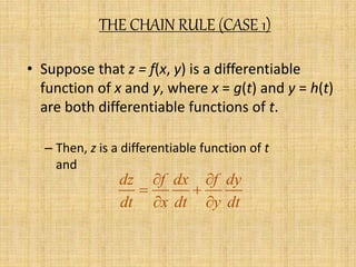
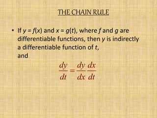
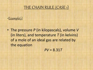
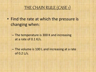
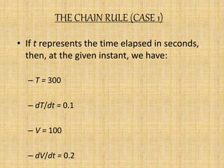
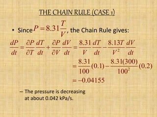
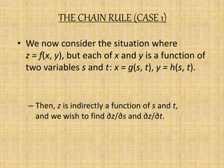
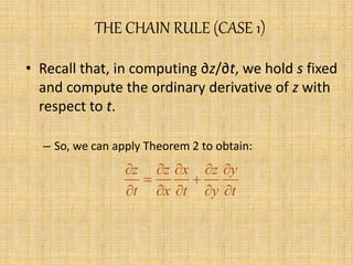
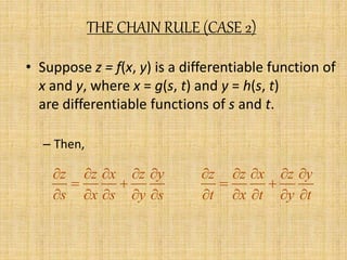
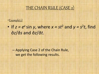
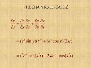
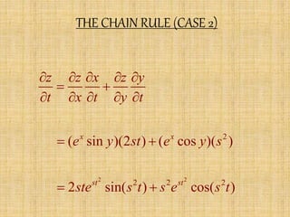
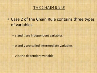
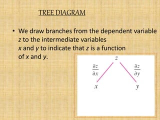
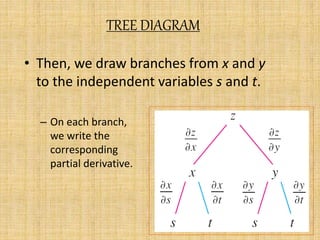
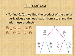
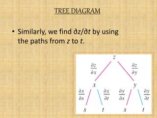
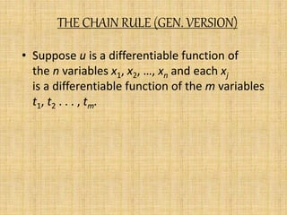
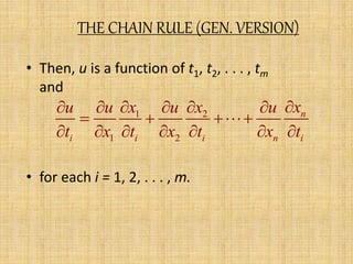
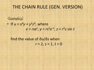
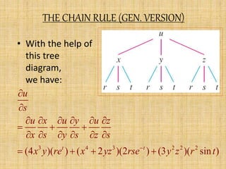
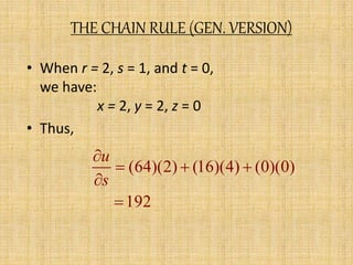
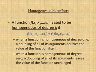
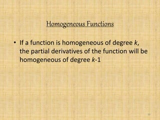
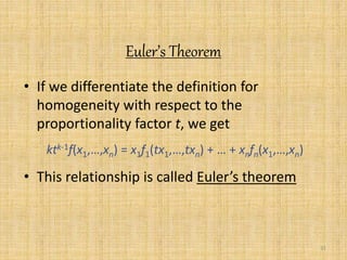
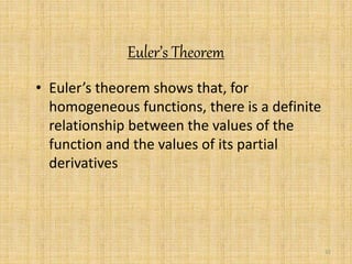
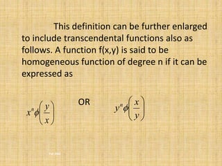
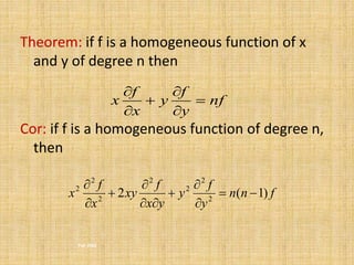
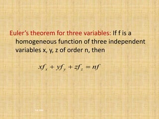
The document discusses the chain rule and Euler's theorem. It explains the chain rule for functions of single, multiple, and general variables. The chain rule gives rules for finding the derivative of a composite function. It also explains that if a function is homogeneous of degree k, its partial derivatives will be homogeneous of degree k-1. Euler's theorem relates the values of a homogeneous function to the values of its partial derivatives. The theorem is extended to functions of multiple variables.

1. G.H.Patel College of
Engineering And Technology
Chain Rule And Euler’s Theoram
Created By
Enrolment number
130110120022 To
130110120028
Tanuj Parikh
Akash Pansuriya

2. The Chain Rule
In this section, we will learn
about:
The Chain Rule

3. thE CHAIN RULE
• Recall that the Chain Rule for functions
of a single variable gives the following rule
for differentiating a composite function.

4. THE CHAIN RULE (CASE 1)
• Suppose that z = f(x, y) is a differentiable
function of x and y, where x = g(t) and y = h(t)
are both differentiable functions of t.
– Then, z is a differentiable function of t
and
dz f dx f dy
dt x dt y dt
 
 
 

5. THE CHAIN RULE
• If y = f(x) and x = g(t), where f and g are
differentiable functions, then y is indirectly
a differentiable function of t,
and
dy dy dx

dt dx dt

6. THE CHAIN RULE
• For functions of more than one variable,
the Chain Rule has several versions.
– Each gives a rule for differentiating
a composite function.

7. -Example(1)
THE CHAIN RULE (CASE 1)
• The pressure P (in kilopascals), volume V
(in liters), and temperature T (in kelvins)
of a mole of an ideal gas are related by
the equation
PV = 8.31T

8. THE CHAIN RULE (CASE 1)
• Find the rate at which the pressure is
changing when:
– The temperature is 300 K and increasing
at a rate of 0.1 K/s.
– The volume is 100 L and increasing at a rate
of 0.2 L/s.

9. THE CHAIN RULE (CASE 1)
• If t represents the time elapsed in seconds,
then, at the given instant, we have:
– T = 300
– dT/dt = 0.1
– V = 100
– dV/dt = 0.2

10. THE CHAIN RULE (CASE 1)
8.31
T
P

• Since , the Chain Rule gives:
V
dP  P dT 
P dV dT T dV
   
dt  T dt 
V dt V dt V dt
 
– The pressure is decreasing
at about 0.042 kPa/s.
2
2
8.31 8.13
8.31 8.31(300)
(0.1) (0.2)
100 100
0.04155
 

11. THE CHAIN RULE (CASE 1)
• We now consider the situation where
z = f(x, y), but each of x and y is a function of
two variables s and t: x = g(s, t), y = h(s, t).
– Then, z is indirectly a function of s and t,
and we wish to find ∂z/∂s and ∂z/∂t.

12. THE CHAIN RULE (CASE 1)
• Recall that, in computing ∂z/∂t, we hold s fixed
and compute the ordinary derivative of z with
respect to t.
– So, we can apply Theorem 2 to obtain:
z z x z y
t x t y t
    
 
    

13. • Suppose z = f(x, y) is a differentiable function of
x and y, where x = g(s, t) and y = h(s, t)
are differentiable functions of s and t.
– Then,
THE CHAIN RULE (CASE 2)
z z x z y z z x z y
s x s y s t x t y t
         
   
         

14. THE CHAIN RULE (CASE 2)
-Example(2)
• If z = ex sin y, where x = st2 and y = s2t, find
∂z/∂s and ∂z/∂t.
– Applying Case 2 of the Chain Rule,
we get the following results.

15. THE CHAIN RULE (CASE 2)
z z x z y
s x s y s
    
 
    
x 2
x
e y t e y st
 
( sin )( ) ( cos )(2 )
2 2
st st
2 2 2
t e s t ste s t
 
sin( ) 2 cos( )

16. THE CHAIN RULE (CASE 2)
z z x z y
t x t y t
x x
2
    
 
    
e y st e y s
 ( sin )(2 ) 
( cos )( )
2 2
st st
2 2 2
ste s t s e s t
 2 sin( ) 
cos( )

17. THE CHAIN RULE
• Case 2 of the Chain Rule contains three types
of variables:
– s and t are independent variables.
– x and y are called intermediate variables.
– z is the dependent variable.

18. THE CHAIN RULE
• To remember the Chain Rule,
it’s helpful to draw a tree diagram,
as follows.

19. TREE DIAGRAM
• We draw branches from the dependent variable
z to the intermediate variables
x and y to indicate that z is a function
of x and y.

20. TREE DIAGRAM
• Then, we draw branches from x and y
to the independent variables s and t.
– On each branch,
we write the
corresponding
partial derivative.

21. TREE DIAGRAM
• To find ∂z/∂s, we find the product of the partial
derivatives along each path from z to s and then
add these products:
z z x z y
s x s y s
    
 
    

22. TREE DIAGRAM
• Similarly, we find ∂z/∂t by using
the paths from z to t.

23. THE CHAIN RULE (GEN. VERSION)
• Suppose u is a differentiable function of
the n variables x1, x2, …, xn and each xj
is a differentiable function of the m variables
t1, t2 . . . , tm.

24. THE CHAIN RULE (GEN. VERSION)
• Then, u is a function of t1, t2, . . . , tm
and
u u x u x u x
t x t x t x t
      
1 2
      
      
1 2
• for each i = 1, 2, . . . , m.
n
i i i n i

25. THE CHAIN RULE (GEN. VERSION)
-Example(3)
• If u = x4y + y2z3, where
x = rset, y = rs2e–t, z = r2s sin t
find the value of ∂u/∂s when
r = 2, s = 1, t = 0

26. THE CHAIN RULE (GEN. VERSION)
• With the help of
this tree
diagram,
we have:
u
s
u x u y u z
x s y s z s


     
  
     
   
(4 x 3 y )( re t ) ( x 4 2 yz 3 )(2 rse 
t
) (3 y 2 z 2 )( r 2 sin t )

27. THE CHAIN RULE (GEN. VERSION)
• When r = 2, s = 1, and t = 0,
we have:
x = 2, y = 2, z = 0
• Thus,
(64)(2) (16)(4) (0)(0)
192
u
s

  



29. 29
Homogeneous Functions
• A function f(x1,x2,…xn) is said to be
homogeneous of degree k if
f(tx1,tx2,…txn) = tk f(x1,x2,…xn)
– when a function is homogeneous of degree one,
a doubling of all of its arguments doubles the
value of the function itself
– when a function is homogeneous of degree
zero, a doubling of all of its arguments leaves
the value of the function unchanged

30. 30
Homogeneous Functions
• If a function is homogeneous of degree k,
the partial derivatives of the function will be
homogeneous of degree k-1

31. 31
Euler’s Theorem
• If we differentiate the definition for
homogeneity with respect to the
proportionality factor t, we get
ktk-1f(x1,…,xn) = x1f1(tx1,…,txn) + … + xnfn(x1,…,xn)
• This relationship is called Euler’s theorem

32. 32
Euler’s Theorem
• Euler’s theorem shows that, for
homogeneous functions, there is a definite
relationship between the values of the
function and the values of its partial
derivatives

33. This definition can be further enlarged
to include transcendental functions also as
follows. A function f(x,y) is said to be
homogeneous function of degree n if it can be
expressed as

Fall 2002
OR



x


y


y
xn  

 

x
yn

34. Theorem: if f is a homogeneous function of x
and y of degree n then
f
f


x 
Cor: if f is a homogeneous function of degree n,
then

Fall 2002
nf
y
y
x



n n f
2
y
f
y
f
2

x y
xy
x
f
2

x 2 ( 1) 2
2
2
2  


 



35. Euler’s theorem for three variables: If f is a
homogeneous function of three independent
variables x, y, z of order n, then
xf yf zf nf x y z   
Fall 2002

36. Modified EULER’s theorem
If Z is a Homogeneous function of degree n in
the variables x and y and z=f(u)
f u
( )
f u
' ( )
n
u


x 
y
y
u
x



If z is a homogeneous function of degree n in
the variables x and y and z=f(u)
2

u
2 ( )[ ' ( ) 1],
u
2
2
2
u
2
2


2  
 




g u g u
x y
xy
y
y
x
x
f u
( )
' ( )
( )
f u
g u  n
where