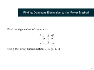
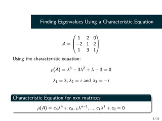
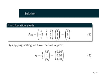
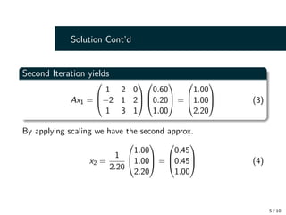
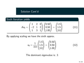
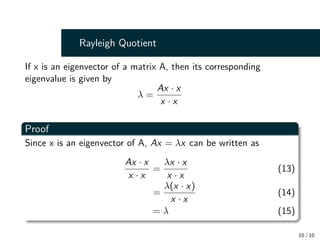
The document discusses using the power method to find the dominant eigenvalue of a 3x3 matrix. It provides the steps of applying the power method to the given matrix, showing the calculations for 6 iterations. The dominant eigenvalue converges to 3. The document also discusses using the Rayleigh quotient to calculate the eigenvalue corresponding to an eigenvector.

1. Isaac Amornortey Yowetu
Approximating a
Dominant Eigenvalue by
the Power Method
March 15, 2022

2. Finding Dominant Eigenvalue by the Power Method
Find the eigenvalues of the matrix



1 2 0
−2 1 2
1 3 1



Using the initail approximation x0 = (1, 1, 1)
2 / 10

3. Finding Eigenvalues Using a Characteristic Equation
A =



1 2 0
−2 1 2
1 3 1



Using the characteristic equation:
ρ(A) = λ3
− 3λ2
+ λ − 3 = 0
λ1 = 3, λ2 = i and λ3 = −i
Characteristic Equation for nxn matrices
ρ(A) = cnλn
+ cn−1λn−1
, ..., c1λ1
+ c0 = 0
3 / 10

4. Solution
First Iteration yields
Ax0 =



1 2 0
−2 1 2
1 3 1






1
1
1


 =



3
1
5


 (1)
By applying scaling we have the first approx.
x1 =
1
5



3
1
5


 =



0.60
0.20
1.00


 (2)
4 / 10

5. Solution Cont’d
Second Iteration yields
Ax1 =



1 2 0
−2 1 2
1 3 1






0.60
0.20
1.00


 =



1.00
1.00
2.20


 (3)
By applying scaling we have the second approx.
x2 =
1
2.20



1.00
1.00
2.20


 =



0.45
0.45
1.00


 (4)
5 / 10

6. Solution Cont’d
Third Iteration yields
Ax2 =



1 2 0
−2 1 2
1 3 1






0.45
0.45
1.00


 =



1.35
1.55
2.80


 (5)
By applying scaling we have the third approx.
x3 =
1
2.80



1.35
1.55
2.80


 =



0.48
0.55
1.00


 (6)
6 / 10

7. Solution Cont’d
Fourth Iteration yields
Ax3 =



1 2 0
−2 1 2
1 3 1






0.48
0.55
1.00


 =



1.58
1.59
3.13


 (7)
By applying scaling we have the fourth approx.
x4 =
1
3.13



1.58
1.59
3.13


 =



0.50
0.51
1.00


 (8)
7 / 10

8. Solution Cont’d
Fifth Iteration yields
Ax4 =



1 2 0
−2 1 2
1 3 1






0.50
0.51
1.00


 =



1.52
1.51
3.03


 (9)
By applying scaling we have the fifth approx.
x5 =
1
3.03



1.52
1.51
3.03


 =



0.50
0.50
1.00


 (10)
8 / 10

9. Solution Cont’d
Sixth Iteration yields
Ax5 =



1 2 0
−2 1 2
1 3 1






0.50
0.50
1.00


 =



1.5
1.5
3.0


 (11)
By applying scaling we have the sixth approx.
x6 =
1
3.0



1.5
1.5
3.0


 =



0.50
0.50
1.00


 (12)
The dominant eigenvalue is: 3
9 / 10

10. Rayleigh Quotient
If x is an eigenvector of a matrix A, then its corresponding
eigenvalue is given by
λ =
Ax · x
x · x
Proof
Since x is an eigenvector of A, Ax = λx can be written as
Ax · x
x · x
=
λx · x
x · x
(13)
=
λ(x · x)
x · x
(14)
= λ (15)
10 / 10