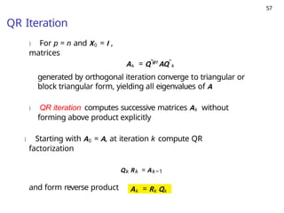
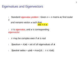
Here's a summary of the eigenvalue problem for a general audience: What is an eigenvalue problem? An eigenvalue problem is a mathematical problem that involves finding a special value (called an eigenvalue) an Eigenvalue problems can be challenging to solve, especially for large matrices. Some of the challenges include finding the eigenvalues and eigenvectors, dealing with non-unique solutions, and handling ill-conditioned matrices.

1. CS 450 – Numerical Analysis
Chapter 4: Eigenvalue Problems
†
Prof. Michael T. Heath
Department of Computer Science
University of Illinois at Urbana-
Champaign heath@illinois.edu
January 28, 2019
†
Lecture slides based on the textbook Scientific Computing: An
Introductory Survey by Michael T. Heath, copyright ⃝c 2018 by the Society
for Industrial and Applied Mathematics. http://www.siam.org/books/cl80

2. 2
Eigenvalue
Problems

3. 3
Eigenvalues and Eigenvectors
) Standard eigenvalue problem : Given n × n matrix A, find scalar
λ
and nonzero vector x such that
Ax = λ x
) λ is eigenvalue, and x is corresponding
eigenvector
) λ may be complex even if A is real
) Spectrum = λ(A) = set of all eigenvalues of A
) Spectral radius = ρ(A) = max{|λ| : λ ∈ λ(A)}

4. 4
Geometric Interpretation
) Matrix expands or shrinks any vector lying in direction of
eigenvector by scalar factor
) Scalar expansion or contraction factor is given by
corresponding eigenvalue λ
) Eigenvalues and eigenvectors decompose complicated
behavior of general linear transformation into simpler
actions

5. 5
Eigenvalue Problems
) Eigenvalue problems occur in many areas of science and
engineering, such as structural analysis
) Eigenvalues are also important in analyzing numerical methods
) Theory and algorithms apply to complex matrices as well
as real matrices
) With complex matrices, we use conjugate transpose, AH ,
instead of usual transpose, AT

6. 6
Examples: Eigenvalues and Eigenvectors
) A =
1 0
0 2 1 1
1
0
: λ = 1, x = , 2 2
λ = 2, x =
0
1
) A =
1 1
0 2 1
1
1
0
: λ = 1, x = , λ2 = 2, x2 =
1
1
) A =
3 —
1
: λ 1 1
= 2, x =
1
1 , λ2 = 4, x2 =
1
—
1
) A =
—1
3
1.5 0.5
0.5 1.5
1
1
1
1
: λ = 2, x = , 2 2
λ = 1, x =
—
1 1
) A =
0 1
—1
0
1
i
1 1 2
2
: λ = i , x = , λ = —i, x =
i
1
where i =
√
—1

7. 7
Characteristic Polynomial and
Multiplicity

8. 8
Characteristic Polynomial
) Equation Ax = λx is equivalent to
(A — λI )x = 0
which has nonzero solution x if, and only if, its matrix is
singular
) Eigenvalues of A are roots λi of characteristic polynomial
det(A — λI ) = 0
in λ of degree n
) Fundamental Theorem of Algebra implies that n × n matrix A
always has n eigenvalues, but they may not be real nor
distinct
) Complex eigenvalues of real matrix occur in complex
conjugate
pairs: if α + iβ is eigenvalue of real matrix, then so is α — iβ,
where
√
i = —
1

9. 9
Example: Characteristic Polynomial
) Characteristic polynomial of previous example
matrix is
de
t
3 —
1
—1
3
—
λ
1 0
0 1
=
de
t
3 — λ —
1—1 3 —
λ
=
2
(3 — λ)(3 — λ) — (—1)(—1) = λ
— 6λ + 8 = 0
so eigenvalues are given by
√
2
1
2
6 ± 36 — 32
λ = , or λ = 2, λ = 4

10. 10
Companion Matrix
) Monic polynomial
p(λ) = c0 + c1λ + · · · + cn− 1λn− 1
+ λn
is characteristic polynomial of companion matrix
n
C =





0 0 · · · 0 —c0
1 0 · · · 0 —c1
0 1 · · · 0 —c2
. .
. . . .. . .
. .
0 0 · · ·
1
—cn−1





) Roots of polynomial of degree > 4 cannot always computed in
finite number of steps
) So in general, computation of eigenvalues of matrices of
order > 4 requires (theoretically infinite) iterative process

11. 11
Characteristic Polynomial, continued
) Computing eigenvalues using characteristic polynomial is not
recommended because of
) work in computing coefficients of characteristic polynomial
) sensitivity of coefficients of characteristic polynomial
) work in solving for roots of characteristic polynomial
) Characteristic polynomial is powerful theoretical tool but
usually not useful computationally

12. 12
Example: Characteristic Polynomial
)
Consider A =
1 ϵ
ϵ
1
where ϵ is positive number slightly smaller than
√
ϵmach
) Exact eigenvalues of A are 1 + ϵ and 1 — ϵ
) Computing characteristic polynomial in floating-point
arithmetic, we obtain
det(A — λI ) = λ2
— 2λ + (1 — ϵ2
) = λ2
— 2λ + 1
which has 1 as double root
) Thus, eigenvalues cannot be resolved by this method even
though they are distinct in working precision

13. 13
Multiplicity and Diagonalizability
) Multiplicity is number of times root appears when
polynomial is written as product of linear factors
) Simple eigenvalue has multiplicity 1
) Defective matrix has eigenvalue of multiplicity k > 1 with
fewer than k linearly independent corresponding
eigenvectors
) Nondefective matrix A has n linearly independent eigenvectors,
so it is diagonalizable
X − 1
AX = D
where X is nonsingular matrix of eigenvectors

14. 14
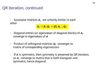
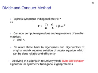
Eigenspaces and Invariant Subspaces
) Eigenvectors can be scaled arbitrarily: if Ax = λx ,
then A(γx ) = λ(γx ) for any scalar γ, so γx is also
eigenvector corresponding to λ
) Eigenvectors are usually normalized by requiring some
norm of eigenvector to be 1
) Eigenspace = Sλ = {x : Ax = λx }
) Subspace S of Rn (or Cn ) is invariant if AS ⊆ S
) For eigenvectors x1 · · · xp , span([x1 · · · xp ]) is invariant
subspace

15. 15
Relevant Properties of
Matrices

16. 16
Relevant Properties of Matrices
) Properties of matrix A relevant to eigenvalue
problems
Property Definition
aij = 0 for i /= j
aij = 0 for |i — j| > 1
diagonal
tridiagon
al
triangula
r
aij = 0 for i > j (upper)
aij = 0 for i < j (lower)
aij = 0 for i > j + 1 (upper)
aij = 0 for i < j — 1 (lower)
AT A = AAT = I
AH A = AAH = I
A = AT
A = AH
AH A = AAH
Hessenber
g
orthogon
al unitary
symmetri
c
Hermitia
n normal

17. 17
Examples: Matrix Properties
)
Transpose:
1 2
3 4
T
=
1 3
2 4
) Conjugate
transpose:
1 + i 1 + 2i
2 — i 2 —
2i
H
=
1 — i 2 + i
1 —
2i
2 + 2i
) Symmetric
:
1 2
2 3
) Nonsymmetri
c:
1 3
2 4
) Hermitian:
1 1
+ i
1 — i 2
) NonHermitian:
1 1 + i
1 + i 2

18. 18
Examples, continued
)
Orthogonal: 0
,
0 1 —
1
1
0
0 —
1 ,
2/2 2/2
—
√
2/2
√
2/2
√ √
)
Unitary:
√
i 2/2 2/2
—
√
2/2 —i
√
2/2
√
) Nonorthogon
al:
1 1
1 2
) 

1 2
Normal: 0 1 2
2 0 1
0


) Nonnorma
l:
1 1
0 1

19. 19
Properties of Eigenvalue Problems
Properties of eigenvalue problem affecting choice of
algorithm and software
) Are all eigenvalues needed, or only a few?
) Are only eigenvalues needed, or are corresponding
eigenvectors also needed?
) Is matrix real or complex?
) Is matrix relatively small and dense, or large and sparse?
) Does matrix have any special properties, such as symmetry,
or is it general matrix?

20. 20
Conditioning of Eigenvalue
Problems

21. 21
Conditioning of Eigenvalue Problems
) Condition of eigenvalue problem is sensitivity of
eigenvalues and eigenvectors to changes in matrix
) Conditioning of eigenvalue problem is not same as
conditioning of solution to linear system for same matrix
) Different eigenvalues and eigenvectors are not necessarily
equally sensitive to perturbations in matrix

22. 22
Conditioning of Eigenvalues
) If µ is eigenvalue of perturbation A + E of nondefective
matrix A, then
|µ — λk | ≤ cond2(X ) E 2
where λk is closest eigenvalue of A to µ and X is nonsingular
matrix of eigenvectors of A
) Absolute condition number of eigenvalues is condition
number of matrix of eigenvectors with respect to solving
linear equations
) Eigenvalues may be sensitive if eigenvectors are nearly
linearly dependent (i.e., matrix is nearly defective)
) For normal matrix (AH A = AAH ), eigenvectors are orthogonal,
so eigenvalues are well-conditioned

23. 23
Conditioning of Eigenvalues
) If (A + E )(x + ∆x ) = (λ + ∆λ)(x + ∆x ), where λ is simple
eigenvalue of A, then
2
|y H x |
cos(θ)
y 2 · x 2
1
|∆λ| € E = E
2
where x and y are corresponding right and left eigenvectors
and θ is angle between them
) For symmetric or Hermitian matrix, right and left
eigenvectors are same, so cos(θ) = 1 and eigenvalues are
inherently well-conditioned
) Eigenvalues of nonnormal matrices may be sensitive
) For multiple or closely clustered eigenvalues,
corresponding eigenvectors may be sensitive

24. 24
Computing Eigenvalues and
Eigenvectors

25. 25
Problem Transformations
) Shift : If Ax = λx and σ is any scalar, then (A — σI )x = (λ — σ)x
, so eigenvalues of shifted matrix are shifted eigenvalues of
original matrix
) Inversion : If A is nonsingular and Ax = λx with x /= 0, then
λ /= 0 and A− 1 x = (1/λ)x , so eigenvalues of inverse are
reciprocals of eigenvalues of original matrix
) Powers : If Ax = λx , then Ak x = λk x , so eigenvalues of power
of matrix are same power of eigenvalues of original matrix
) Polynomial : If Ax = λx and p(t) is polynomial, then
p(A)x = p(λ)x , so eigenvalues of polynomial in matrix are values of
polynomial evaluated at eigenvalues of original matrix

26. 26
Similarity Transformation
) B is similar to A if there is nonsingular matrix T such
that
B = T − 1 A T
) Then
By = λy ⇒ T − 1
ATy = λy ⇒ A(Ty ) = λ(Ty )
so A and B have same eigenvalues, and if y is eigenvector of
B, then x = Ty is eigenvector of A
) Similarity transformations preserve eigenvalues, and
eigenvectors are easily recovered

27. 27
Example: Similarity Transformation
) From eigenvalues and eigenvectors for previous
example,
3 —1 1
1
—1 3 1 —
1
=
1 1 2 0
1 —1 0 4
and
hence
0.5 0.5 3 —1 1
1
0.5 —0.5 —1 3 1 —
1
=
2 0
0 4
) So original matrix is similar to diagonal matrix, and
eigenvectors form columns of similarity transformation
matrix

28. 28
Diagonal
Form
) Eigenvalues of diagonal matrix are diagonal entries, and
eigenvectors are columns of identity matrix
) Diagonal form is desirable in simplifying eigenvalue
problems for general matrices by similarity transformations
) But not all matrices are diagonalizable by similarity
transformation
) Closest one can get, in general, is Jordan form, which is nearly
diagonal but may have some nonzero entries on first
superdiagonal, corresponding to one or more multiple
eigenvalues

29. 29
Triangular
Form
) Any matrix can be transformed into triangular (Schur ) form
by similarity, and eigenvalues of triangular matrix are
diagonal entries
) Eigenvectors of triangular matrix less obvious, but
still straightforward to compute
) If


U11
u
A — λI = 0 0 vT
O 0
U33
U13


is triangular, then U11y = u can be solved for y , so
that

y

x = —1
 
0
is corresponding eigenvector

30. 30
Block Triangular
Form
)
If
A =



A1
1 A12

1p
· · · A
· · · A
A22
2p
. .. .
.




App
with square diagonal blocks, then
p
[
λ(A) = λ(A
j=1
so eigenvalue problem breaks into p smaller eigenvalue
problems
) Real Schur form has 1 × 1 diagonal blocks corresponding
to real eigenvalues and 2 × 2 diagonal blocks corresponding
to pairs of complex conjugate eigenvalues
jj )

31. 31
Forms Attainable by Similarity
A T B
distinct
eigenvalues real
symmetric
complex
Hermitian normal
arbitrary real
nonsingula
r
orthogona
l unitary
unitary
orthogona
l
diagonal
real
diagonal
real
diagonal
diagonal
real block
triangular (real
Schur)
upper
triangular
(Schur)
almost
diagonal
(Jordan)
arbitrar
y
unitar
y
arbitrar
y
nonsingula
r
) Given matrix A with indicated property, matrices B and T
exist with indicated properties such that B = T − 1 AT
) If B is diagonal or triangular, eigenvalues are its diagonal
entries
) If B is diagonal, eigenvectors are columns of T

32. 32
Power
Iteration

33. 33
Power Iteration
) Simplest method for computing one eigenvalue-eigenvector
pair is power iteration, which repeatedly multiplies matrix
times initial starting vector
) Assume A has unique eigenvalue of maximum modulus, say λ1,
with corresponding eigenvector v1
) Then, starting from nonzero vector x0, iteration scheme
xk = Axk − 1
converges to multiple of eigenvector v1 corresponding to
dominant
eigenvalue λ1

34. 34
Convergence of Power Iteration
) To see why power iteration converges to dominant
eigenvector, express starting vector x0 as linear
combination
n
Σ
x = α v
0 i i
i=1
where vi are eigenvectors of A
) Then
xk = Axk − 1 = A2
xk − 2 = · · · = Ak
x0 =
n
Σ
i=1
i
1
n
Σ
λk
αi vi = λk
α1v1 + (λi /λ1)k
αi vi
i=2
!
) Since |λi /λ1 | < 1 for i > 1, successively higher powers go to
zero, leaving only component corresponding to v1

35. 35
Example: Power Iteration
) Ratio of values of given component of xk from one iteration to
next converges to dominant eigenvalue λ1
) For example, if A
=
1.5 0.5
0.5 1.5 0
0
1
and x = , we
obtain
k x T
k rati
o
0 0.0 1.0
1 0.5 1.5 1.500
2 1.5 2.5 1.667
3 3.5 4.5 1.800
4 7.5 8.5 1.889
5 15.5 16.5 1.941
6 31.5 32.5 1.970
7 63.5 64.5 1.985
8 127.5 128.5 1.992
) Ratio is converging to dominant eigenvalue, which
is 2

36. 36
Limitations of Power Iteration
Power iteration can fail for various reasons
) Starting vector may have no component in dominant
eigenvector v1 (i.e., α1 = 0) — not problem in practice because
rounding error usually introduces such component in any case
) There may be more than one eigenvalue having same
(maximum) modulus, in which case iteration may converge to
linear combination of corresponding eigenvectors
) For real matrix and starting vector, iteration can never
converge to complex vector

37. 37
Normalized Power Iteration
) Geometric growth of components at each iteration risks
eventual overflow (or underflow if λ1 < 1)
) Approximate eigenvector should be normalized at each
iteration, say, by requiring its largest component to be 1 in
modulus, giving iteration scheme
Axk−1
yk =
xk = yk / yk ∞
) With normalization, yk ∞ → |λ1|, and xk → v1 / v1
∞

38. 38
Example: Normalized Power Iteration
) Repeating previous example with normalized
scheme,
k x T
k yk ∞
0 0.000 1.0
1 0.333 1.0 1.500
2 0.600 1.0 1.667
3 0.778 1.0 1.800
4 0.882 1.0 1.889
5 0.939 1.0 1.941
6 0.969 1.0 1.970
7 0.984 1.0 1.985
8 0.992 1.0 1.992
⟨ interactive example
⟩

39. 39
Geometric Interpretation
) Behavior of power iteration depicted
geometrically
) Initial vector x0 = v1 + v2 contains equal components
in eigenvectors v1 and v2 (dashed arrows)
) Repeated multiplication by A causes component in v1
(corresponding to larger eigenvalue, 2) to dominate, so
sequence of vectors xk converges to v1

40. 40
Power Iteration with Shift
) Convergence rate of power iteration depends on ratio |λ2/λ1|,
where
λ2 is eigenvalue having second largest modulus
) May be possible to choose shift, A — σI , such that
2
1
λ —
σ
<
λ — σ λ2
λ1
so convergence is accelerated
) Shift must then be added to result to obtain eigenvalue of
original matrix
) In earlier example, for instance, if we pick shift of σ = 1,
(which is equal to other eigenvalue) then ratio becomes zero
and method converges in one iteration
) In general, we would not be able to make such fortuitous
choice, but shifts can still be extremely useful in some contexts,
as we will see later

41. 41
Inverse and Rayleigh Quotient
Iterations

42. 42
Inverse Iteration
) To compute smallest eigenvalue of matrix rather than largest,
can make use of fact that eigenvalues of A− 1 are reciprocals of
those of A, so smallest eigenvalue of A is reciprocal of largest
eigenvalue of
A−1
) This leads to inverse iteration scheme
xk−1
Ayk =
xk = yk / yk
∞
which is equivalent to power iteration applied to A− 1
) Inverse of A not computed explicitly, but factorization of A
used to solve system of linear equations at each iteration
) Inverse iteration converges to eigenvector corresponding to
smallest
eigenvalue of A
) Eigenvalue obtained is dominant eigenvalue of A− 1 , and

43. 43
Example: Inverse Iteration
) Applying inverse iteration to previous example to compute
smallest eigenvalue yields sequence
k x T
k yk ∞
0 0.000 1.0
1 —0.333 1.0
0.750
2 —0.600 1.0
0.833
3 —0.778 1.0
0.900
4 —0.882 1.0
0.944
5 —0.939 1.0
0.971
6 —0.969 1.0
0.985
which is indeed converging to 1 (which is its own reciprocal in

44. 44
Inverse Iteration with Shift
) As before, shifting strategy, working with A — σI for some
scalar σ, can greatly improve convergence
) Inverse iteration is particularly useful for computing
eigenvector corresponding to approximate eigenvalue, since it
converges rapidly when applied to shifted matrix A — λI ,
where λ is approximate eigenvalue
) Inverse iteration is also useful for computing eigenvalue
closest to given value β, since if β is used as shift, then
desired eigenvalue corresponds to smallest eigenvalue of
shifted matrix

45. 45
Rayleigh
Quotient
) Given approximate eigenvector x for real matrix A, determining
best estimate for corresponding eigenvalue λ can be considered
as n × 1 linear least squares approximation problem
x λ ∼= Ax
) From normal equation x T x λ = x T Ax, least squares solution is
given by
λ =
x T Ax
x T x
) This quantity, known as Rayleigh quotient, has many
useful properties

46. 46
Example: Rayleigh Quotient
) Rayleigh quotient can accelerate convergence of iterative
methods k k
such as power iteration, since Rayleigh quotient x T Axk /x T xk
gives
better approximation to eigenvalue at iteration k than does
basic method alone
) For previous example using power iteration, value of
Rayleigh quotient at each iteration is shown below
k x T
k yk ∞
x T Axk /x T xk
k k
0 0.000 1.0
1 0.333 1.0 1.500 1.500
2 0.600 1.0 1.667 1.800
3 0.778 1.0 1.800 1.941
4 0.882 1.0 1.889 1.985
5 0.939 1.0 1.941 1.996
6 0.969 1.0 1.970 1.999

47. 47
Rayleigh Quotient Iteration
) Given approximate eigenvector
, Rayleigh quotient yields
good estimate for corresponding eigenvalue
) Conversely, inverse iteration converges rapidly to
eigenvector if approximate eigenvalue is used as shift, with
one iteration often sufficing
) These two ideas combined in Rayleigh quotient iteration
σk = x T
Axk /x T
xk
k k
(A — σk I )yk+1 = xk
xk+1 = yk+1/ yk+1 ∞
starting from given nonzero vector x0

48. 48
Rayleigh Quotient Iteration, continued
) Rayleigh quotient iteration is especially effective for
symmetric matrices and usually converges very rapidly
) Using different shift at each iteration means matrix must be
refactored each time to solve linear system, so cost per
iteration is high unless matrix has special form that makes
factorization easy
) Same idea also works for complex matrices, for which
transpose is replaced by conjugate transpose, so Rayleigh
quotient becomes x H Ax/x H x

49. 49
Example: Rayleigh Quotient Iteration
) Using same matrix as previous examples and randomly
chosen starting vector x0, Rayleigh quotient iteration
converges in two iterations
k x T
k σk
0 0.807 0.397 1.896
1 0.924 1.000 1.998
2 1.000 1.000 2.000

50. 50
Deflatio
n

51. 51
Deflation
) After eigenvalue λ1 and corresponding eigenvector x1 have
been computed, then additional eigenvalues λ2, . . . , λn of A
can be computed by deflation, which effectively removes known
eigenvalue
) Let H be any nonsingular matrix such that Hx1 = αe1,
scalar multiple of first column of identity matrix
(Householder transformation is good choice for H)
) Then similarity transformation determined by H transforms
A into form
HAH− 1
=
1
λ bT
0 B
where B is matrix of order n — 1 having eigenvalues λ2, . . .
, λn

52. 52
Deflation, continued
) Thus, we can work with B to compute next eigenvalue λ2
) Moreover, if y2 is eigenvector of B corresponding to λ2,
then
x2 = H −1
, where α =
α bT y2
y2 λ2 —
λ1
is eigenvector corresponding to λ2 for original matrix A,
provided
λ1 /= λ2
) Process can be repeated to find additional
eigenvalues and eigenvectors

53. 53
Deflation, continued
1
) Alternative approach lets u1 be any vector such that uT x1 =
λ1
) 1
T
1
Then A — x u has eigenvalues 0, λ , . . .
, λ
2 n
) Possible choices for u1 include
) u1 = λ1x1, if A is symmetric and x1 is normalized so that x1 2 = 1
) u1 = λ1y1, where y1 is corresponding left eigenvector (i.e.,
1
AT
y1 = λ1y1) normalized so that y T
x1 = 1
) u1 = AT
ek , if x1 is normalized so that x1 ∞ = 1 and
kth component of x1 is 1

54. 54
QR
Iteration

55. 55
Simultaneous Iteration
) Simplest method for computing many eigenvalue-eigenvector
pairs is simultaneous iteration, which repeatedly multiplies matrix
times matrix of initial starting vectors
) Starting from n × p matrix X0 of rank p, iteration scheme is
Xk = AXk − 1
) span(Xk ) converges to invariant subspace determined by p
largest eigenvalues of A, provided |λp | > |λp+1|
) Also called subspace iteration

56. 56
Orthogonal Iteration
) As with power iteration, normalization is needed with
simultaneous iteration
) Each column of Xk converges to dominant eigenvector, so
columns of Xk become increasingly ill-conditioned basis for
span(Xk )
) Both issues can be addressed by computing QR factorization at
each iteration
Qˆk Rk
= Xk−1
Xk =
AQˆk
where Qˆk Rk is reduced QR factorization of Xk − 1
) This orthogonal iteration converges to block triangular form,
and leading block is triangular if moduli of consecutive
eigenvalues are distinct

57. 57
QR Iteration
) For p = n and X0 = I ,
matrices
k
Ak = QˆH
AQˆk
generated by orthogonal iteration converge to triangular or
block triangular form, yielding all eigenvalues of A
) QR iteration computes successive matrices Ak without
forming above product explicitly
) Starting with A0 = A, at iteration k compute QR
factorization
Qk Rk = Ak−1
and form reverse product Ak = Rk Qk

58. 58
QR Iteration, continued
) Successive matrices Ak are unitarily similar to each
other
k
Ak = Rk Qk = QH Ak − 1 Qk
) Diagonal entries (or eigenvalues of diagonal blocks) of Ak
converge to eigenvalues of A
) Product of orthogonal matrices Qk converges to
matrix of corresponding eigenvectors
) If A is symmetric, then symmetry is preserved by QR iteration,
so Ak converge to matrix that is both triangular and
symmetric, hence diagonal

59. 59
Example: QR Iteration
) 0
Let A =
7 2
2 4
) Compute QR
factorization
0 1 1
A = Q R =
.962 —.275
7.28
.275
3.02
.962 0 3.30
and form reverse
product
1 1 1
A = R Q =
7.83 .906
.906 3.17
) Off-diagonal entries are now smaller, and diagonal entries
closer to eigenvalues, 8 and 3
) Process continues until matrix is within tolerance of being
diagonal, and diagonal entries then closely approximate
eigenvalues

60. 60
QR Iteration with
Shifts
) Convergence rate of QR iteration can be
accelerated by incorporating shifts
Qk Rk =
Ak − 1 — σk I Ak =
Rk Qk + σk I
where σk is rough approximation to
eigenvalue
) Good shift can be determined by computing eigenvalues of
2 × 2 submatrix in lower right corner of matrix

61. 61
Example: QR Iteration with Shifts
) Repeat previous example, but with shift of σ1 = 4, which is
lower right corner entry of matrix
) We compute QR factorization
A0 — σ1I = Q1R1 =
.832 .555
3.61
.555
—.832
0
1.6
6
1.1
1
and form reverse product, adding back shift to
obtain
1 1 1
1
A = R Q + σ I =
7.92 .615
.615 3.08
) After one iteration, off-diagonal entries smaller compared
with unshifted algorithm, and diagonal entries closer
approximations to eigenvalues
⟨ interactive example ⟩

62. 62
Preliminary Reduction
) Efficiency of QR iteration can be enhanced by first
transforming matrix as close to triangular form as possible
before beginning iterations
) Hessenberg matrix is triangular except for one additional
nonzero diagonal immediately adjacent to main diagonal
) Any matrix can be reduced to Hessenberg form in finite
number of steps by orthogonal similarity transformation, for
example using Householder transformations
) Symmetric Hessenberg matrix is tridiagonal
) Hessenberg or tridiagonal form is preserved during
successive QR iterations

63. 63
Preliminary Reduction, continued
Advantages of initial reduction to upper Hessenberg or tridiagonal
form
) Work per QR iteration is reduced from O(n3) to O(n2) for
general matrix or O(n) for symmetric matrix
) Fewer QR iterations are required because matrix nearly
triangular (or diagonal) already
) If any zero entries on first subdiagonal, then matrix is
block triangular and problem can be broken into two or
more smaller subproblems
⟨ interactive example ⟩

64. 64
Preliminary Reduction, continued
) QR iteration is implemented in two-stages
symmetric —→ tridiagonal —→
diagonal
or
general —→ Hessenberg —→
triangular
) Preliminary reduction requires definite number of steps,
whereas subsequent iterative stage continues until
convergence
) In practice only modest number of iterations usually
required, so much of work is in preliminary reduction

65. 65
Cost of QR Iteration
Approximate overall cost of preliminary reduction and QR
iteration, counting both additions and multiplications
) Symmetric matrices
) 4
n3
for eigenvalues
only
3
) 9n3
for eigenvalues and
eigenvectors
) General matrices
) 10n3
for eigenvalues only
) 25n3
for eigenvalues and
eigenvectors

66. 66
Krylov Subspace
Methods

67. 67
Krylov Subspace
Methods
) Krylov subspace methods reduce matrix to
Hessenberg (or tridiagonal) form using only matrix-
vector multiplication
) For arbitrary starting vector x0, if
Kk = x0 Ax0 · ·
·
Ak−1x0
the
n n
K − 1
AKn = Cn
where Cn is upper Hessenberg (in fact, companion matrix)
) To obtain better conditioned basis for span(Kn ), compute
QR factorization
Qn Rn = Kn
so that
n n n n
H −1
n
Q AQ = R C R ≡ H
with H upper
Hessenberg

68. 68
Krylov Subspace
Methods
) Equating kth columns on each side of equation AQn = Qn H
yields recurrence
Aqk = h1k q1 + · · · + hkk qk + hk+1,k qk+1
relating qk+1 to preceding vectors q1, . . . , qk
j
) Premultiplying by qH and using
orthonormality,
j
hjk = qH
Aqk , j = 1, . . . ,
k
) These relationships yield Arnoldi iteration, which produces
unitary matrix Qn and upper Hessenberg matrix Hn column by
column using only matrix-vector multiplication by A and inner
products of vectors

69. 69
Arnoldi Iteration
x0 = arbitrary nonzero starting
vector
q1 = x0 / x0 2
for k = 1, 2, . . .
uk = Aqk
for j = 1 to k
j
hjk = qH uk
uk = uk — hjk qj
end
hk+1,k = uk 2
if hk+1,k = 0 then stop
qk+1 = uk /hk+1,k
end

70. 70
Arnoldi Iteration, continued
)
If Qk = q1 · ·
·
qk
the
n k
Hk = QH
AQk
is upper Hessenberg matrix
) Eigenvalues of Hk , called Ritz values, are approximate
eigenvalues of A, and Ritz vectors given by Qk y , where y is
eigenvector of Hk , are corresponding approximate eigenvectors
of A
) Eigenvalues of Hk must be computed by another method,
such as QR iteration, but this is easier problem if k n

71. 71
Arnoldi Iteration, continued
) Arnoldi iteration fairly expensive in work and storage because
each new vector qk must be orthogonalized against all
previous columns of Qk , and all must be stored for that
purpose.
) So Arnoldi process usually restarted periodically with
carefully chosen starting vector
) Ritz values and vectors produced are often good
approximations to eigenvalues and eigenvectors of A after
relatively few iterations

72. 72
Lanczos Iteration
) Work and storage costs drop dramatically if matrix is
symmetric or Hermitian, since recurrence then has only three
terms and Hk is tridiagonal (so usually denoted Tk )
q0 = 0
β0 = 0
x0 = arbitrary nonzero starting vector
q1 = x0 / x0 2
for k = 1, 2, . . .
uk = Aqk
k
αk = qH uk
uk = uk — βk−1qk−1 — αk qk
βk = uk 2
if βk = 0 then stop
qk+1 = uk /βk
end

73. 73
Lanczos Iteration, continued
) αk and βk are diagonal and subdiagonal entries of
symmetric tridiagonal matrix Tk
) As with Arnoldi, Lanczos iteration does not produce
eigenvalues and eigenvectors directly, but only tridiagonal
matrix Tk , whose eigenvalues and eigenvectors must be
computed by another method to obtain Ritz values and vectors
) If βk = 0, then algorithm appears to break down, but in that
case invariant subspace has already been identified (i.e., Ritz
values and vectors are already exact at that point)

74. 74
Lanczos Iteration, continued
) In principle, if Lanczos algorithm were run until k = n,
resulting tridiagonal matrix would be orthogonally similar
to A
) In practice, rounding error causes loss of orthogonality,
invalidating this expectation
) Problem can be overcome by reorthogonalizing vectors as
needed, but expense can be substantial
) Alternatively, can ignore problem, in which case algorithm
still produces good eigenvalue approximations, but multiple
copies of some eigenvalues may be generated

75. 75
Krylov Subspace Methods, continued
) Great virtue of Arnoldi and Lanczos iterations is their
ability to produce good approximations to extreme
eigenvalues for k n
) Moreover, they require only one matrix-vector multiplication
by A per step and little auxiliary storage, so are ideally suited
to large sparse matrices
) If eigenvalues are needed in middle of spectrum, say near σ,
then algorithm can be applied to matrix (A — σI )−1,
assuming it is practical to solve systems of form (A — σI )x =
y

76. 76
Example: Lanczos
Iteration
) For 29 × 29 symmetric matrix with eigenvalues 1, . . . , 29,
behavior of Lanczos iteration is shown below

77. 77
Jacobi
Method

78. 78
Jacobi Method
) One of oldest methods for computing eigenvalues is Jacobi
method, which uses similarity transformation based on plane
rotations
) Sequence of plane rotations chosen to annihilate symmetric
pairs of matrix entries, eventually converging to diagonal form
) Choice of plane rotation slightly more complicated than in
Givens method for QR factorization
) To annihilate given off-diagonal pair, choose c and s so that
J T
AJ =
c —s
a
b
c
s s
c b d —s
c
=
2
2
c2a — 2csb + s2d c b + cs(a — d ) — s
b
c2b + cs(a — d ) —
s2b
c2d + 2csb + s2a
is
diagonal

79. 79
Jacobi Method, continued
) Transformed matrix diagonal if
c2
b + cs(a — d ) — s2
b = 0
) Dividing both sides by c2b, we obtain
1 +
s (a — d )
c
b
s2
—
c2
= 0
) Making substitution t = s/c, we get quadratic
equation
1 + t
(a —
d )
b
2
— t = 0
for
tangen
t t of angle of rotation, from which we can
recover
√
c = 1/( 1 + t2) and s = c · t
) Advantageous numerically to use root of smaller
magnitude

80. 80
Example: Plane Rotation
) Consider 2 × 2
matrix A =
1 2
2 1
) Quadratic equation for tangent reduces to t2 = 1, so t =
±1
) Two roots of same magnitude, so we a rbitrarily choose t =
—1,
√ √
which yields c = 1/ 2 and s = —1/
2
) Resulting plane rotation J
gives
J T
AJ = —1/
√
2 1/
√
2
2 1
1/
√
2 1/ 2 1 2 1/ 2 —1/
2 1/
√
2 1/
√
2
√ √ √
=
3
0
0 —
1

81. 81
Jacobi Method, continued
) Starting with symmetric matrix A0 = A, each iteration has
form
k
Ak +1 = J T
Ak Jk
where Jk is plane rotation chosen to annihilate a symmetric
pair of entries in Ak
) Plane rotations repeatedly applied from both sides in
systematic sweeps through matrix until off-diagonal mass of
matrix is reduced to within some tolerance of zero
) Resulting diagonal matrix orthogonally similar to original
matrix, so diagonal entries are eigenvalues, and eigenvectors
are given by product of plane rotations

82. 82
Jacobi Method, continued
) Jacobi method is reliable, simple to program, and capable of
high accuracy, but converges rather slowly and difficult to
generalize beyond symmetric matrices
) Except for small problems, more modern methods usually
require 5 to 10 times less work than Jacobi
) One source of inefficiency is that previously annihilated
entries can subsequently become nonzero again, thereby
requiring repeated annihilation
) Newer methods such as QR iteration preserve zero
entries introduced into matrix

83. 83
Example: Jacobi Method
) 0
0
Let A = 0 2 1

1 2

 
2 1 1
) First annihilate (1,3) and (3,1) entries using
rotation
J0 =  0
0
0.707 0 —
0.707
1
0.707 0
0.707
 

to
obtain
T
1 0 0
0


3 0
A = J A J = 0.707
0.707
2
0.707
0 0.707 —1



84. 84
Example, continued
) Next annihilate (1,2) and (2,1) entries using
rotation
1


0.888 —0.460
J = 0.460 0.888
0
0

0 0
1

to
obtain
T
2 1 1
1


A = J A J =
0
1.634
0.628
3.366 0 0.325


0.325 0.628
—1
) Next annihilate (2,3) and (3,2) entries using
rotation
2
0
0
J = 0 0.975 —
0.221
0 0.221
0.975

1

 
to
obtain
T
3 2 2
2


3.366
A = J A J = 0.072
0.072
0.317
1.776



85. 85
Example, continued
) Beginning new sweep, again annihilate (1,3) and (3,1) entries
using rotation
J3 =  0
0.998 0 —
0.070
1
0
0.070 0
0.998
 

to
obtain
T
4 3 3
3


3.388
A = J A J = 0.072
0.072 0
1.776 —
0.005


0
—0.005 —1.164
) Process continues until off-diagonal entries reduced to as
small as desired
) Result is diagonal matrix orthogonally similar to original
matrix, with the orthogonal similarity transformation given by
product of plane rotations

86. 86
Other Methods for Symmetric
Matrices

87. 87
Bisection or Spectrum-
Slicing
) For real symmetric matrix, we can determine how many
eigenvalues are less than given real number σ
) By systematically choosing various values for σ (slicing spectrum
at σ) and monitoring resulting count, any eigenvalue can be
isolated as accurately as desired
) For example, symmetric indefinite factorization A = LDLT
makes inertia (numbers of positive, negative, and zero
eigenvalues) of symmetric matrix A easy to determine
) By applying factorization to matrix A — σI for various values
of σ, individual eigenvalues can be isolated as accurately as
desired using interval bisection technique

88. 88
Sturm Sequence
) Another spectrum-slicing method for computing
individual eigenvalues is based on Sturm sequence
property of symmetric matrices
) Let A be symmetric matrix and let pr (σ) denote
determinant of leading principal minor of order r of A — σI
) Then zeros of pr (σ) strictly separate those of pr−1(σ), and
number of agreements in sign of successive members of
sequence pr (σ), for r = 1, . . . , n, equals number of eigenvalues
of A strictly greater than σ
) This property allows computation of number of eigenvalues
lying in any given interval, so individual eigenvalues can be
isolated as accurately as desired
) Determinants pr (σ) are easy to compute if A is
transformed to tridiagonal form before applying Sturm
sequence technique

89. 89
Divide-and-Conquer Method
) Express symmetric tridiagonal matrix T
as
T = 1
T O
O T2
+ β uu T
) Can now compute eigenvalues and eigenvectors of smaller
matrices
T1 and T2
) To relate these back to eigenvalues and eigenvectors of
original matrix requires solution of secular equation, which
can be done reliably and efficiently
) Applying this approach recursively yields divide-and-conquer
algorithm for symmetric tridiagonal eigenproblems

90. 90
Relatively Robust Representation
) With conventional methods, cost of computing
eigenvalues of symmetric tridiagonal matrix is O(n2), but
if orthogonal eigenvectors are also computed, then cost
rises to O(n3)
) Another possibility is to compute eigenvalues first at O(n2)
cost, and then compute corresponding eigenvectors
separately using inverse iteration with computed eigenvalues
as shifts
) Key to making this idea work is computing eigenvalues and
corresponding eigenvectors to very high relative accuracy so
that expensive explicit orthogonalization of eigenvectors is
not needed
) RRR algorithm exploits this approach to produce eigenvalues

91. 91
Generalized Eigenvalue Problems and
SVD

92. 92
Generalized Eigenvalue Problems
) Generalized eigenvalue problem has
form
Ax = λBx
where A and B are given n × n matrices
) If either A or B is nonsingular
, then generalized eigenvalue
problem can be converted to standard eigenvalue problem,
either
(B− 1
A)x = λx or (A− 1
B)x =
(1/λ)x
) This is not recommended,
since it may cause
) loss of accuracy due to rounding
error
) loss of symmetry if A and B are symmetric

93. 93
QZ Algorithm
) If A and B are triangular, then eigenvalues are given by λi =
aii /bii , for bii /= 0
) QZ algorithm reduces A and B simultaneously to upper
triangular form by orthogonal transformations
) First, B is reduced to upper triangular form by
orthogonal transformation from left, which is also
applied to A
) Next, transformed A is reduced to upper Hessenberg form
by orthogonal transformation from left, while maintaining
triangular form of B, which requires additional
transformations from right
) Finally, analogous to QR iteration, A is reduced to triangular
form while still maintaining triangular form of B, which again
requires transformations from both sides
) Eigenvalues can now be determined from mutually triangular

94. 94
Computing SVD
) Singular values of A are nonnegative square roots of
eigenvalues of AT A, and columns of U and V are orthonormal
eigenvectors of AAT and AT A, respectively
) Algorithms for computing SVD work directly with A, without
forming AAT or AT A, to avoid loss of information associated
with forming these matrix products explicitly
) SVD is usually computed by variant of QR iteration, with A
first reduced to bidiagonal form by orthogonal
transformations, then remaining off-diagonal entries are
annihilated iteratively
) SVD can also be computed by variant of Jacobi method, which
can be useful on parallel computers or if matrix has special
structure

95. 95
Summary – Computing Eigenvalues and
Eigenvectors
) Algorithms for computing eigenvalues and
eigenvectors are necessarily iterative
) Power iteration and its variants approximate
one eigenvalue-eigenvector pair
) QR iteration transforms matrix to triangular form by
orthogonal similarity, producing all eigenvalues and
eigenvectors simultaneously
) Preliminary orthogonal similarity transformation to
Hessenberg or tridiagonal form greatly enhances efficiency
of QR iteration
) Krylov subspace methods (Lanczos, Arnoldi) are especially
useful for computing eigenvalues of large sparse matrices
) Many specialized algorithms are available for computing
eigenvalues of real symmetric or complex Hermitian matrices