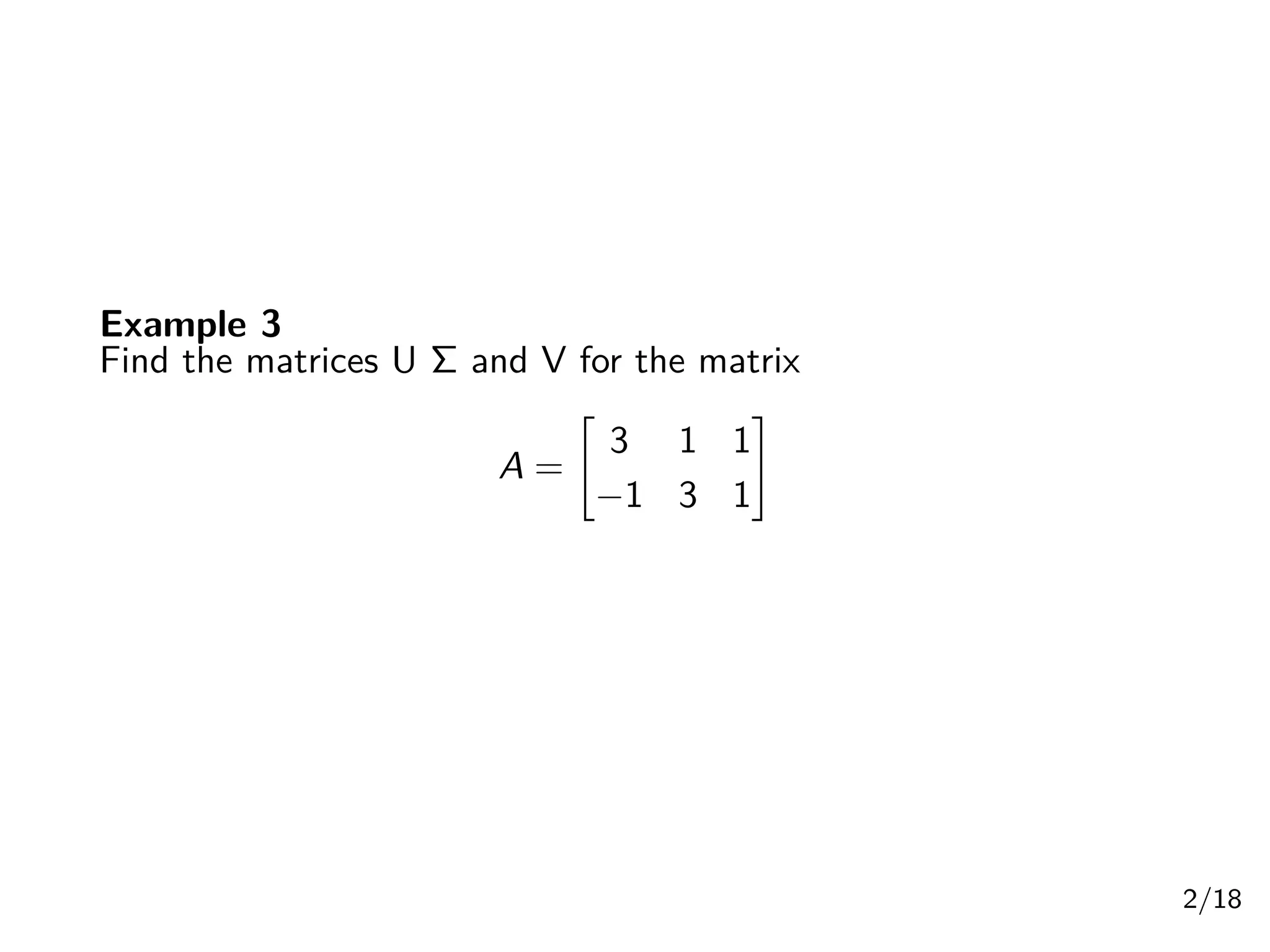
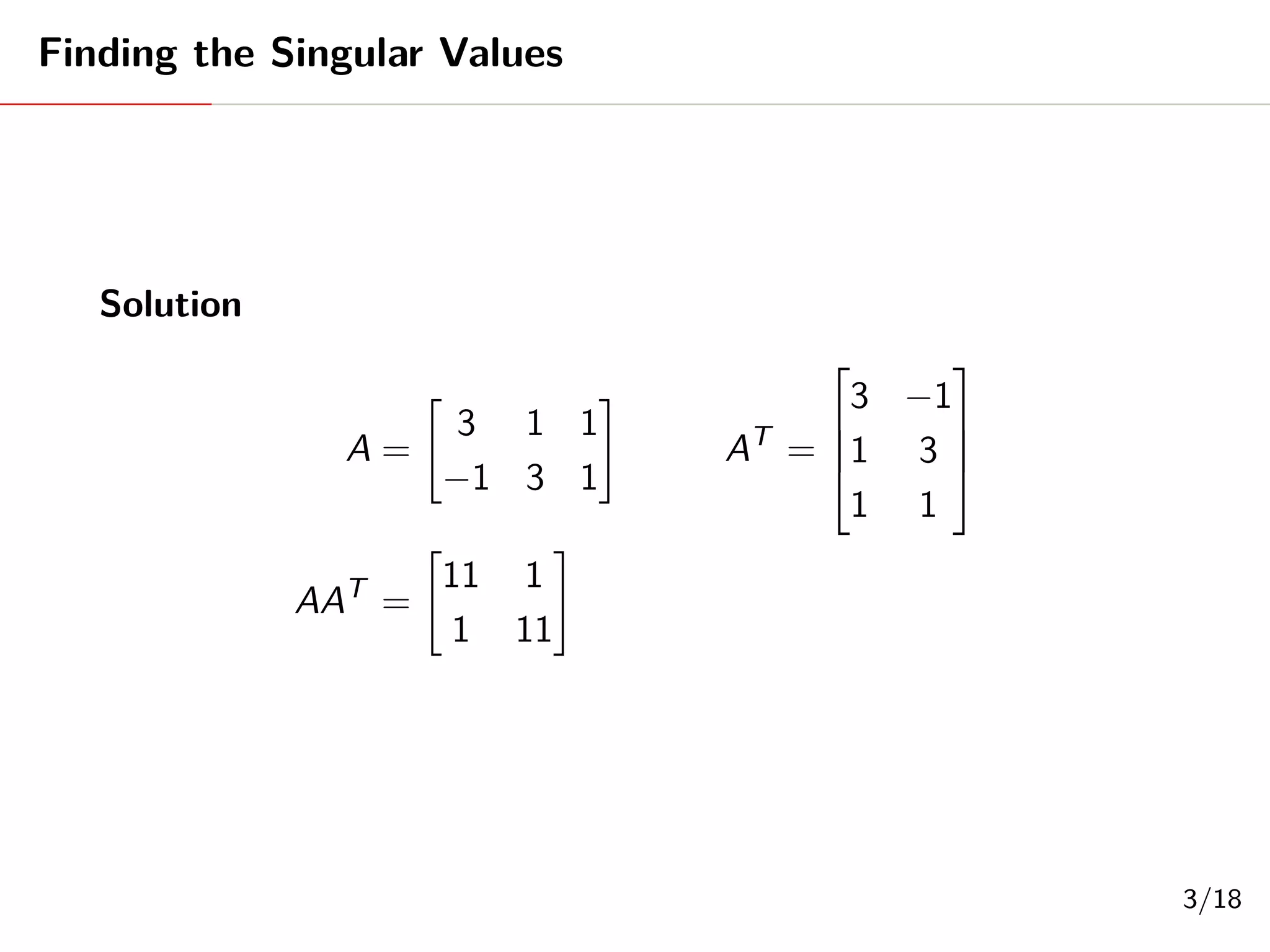
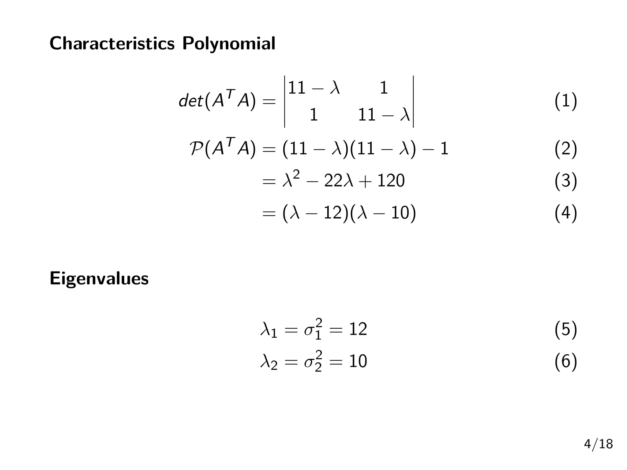
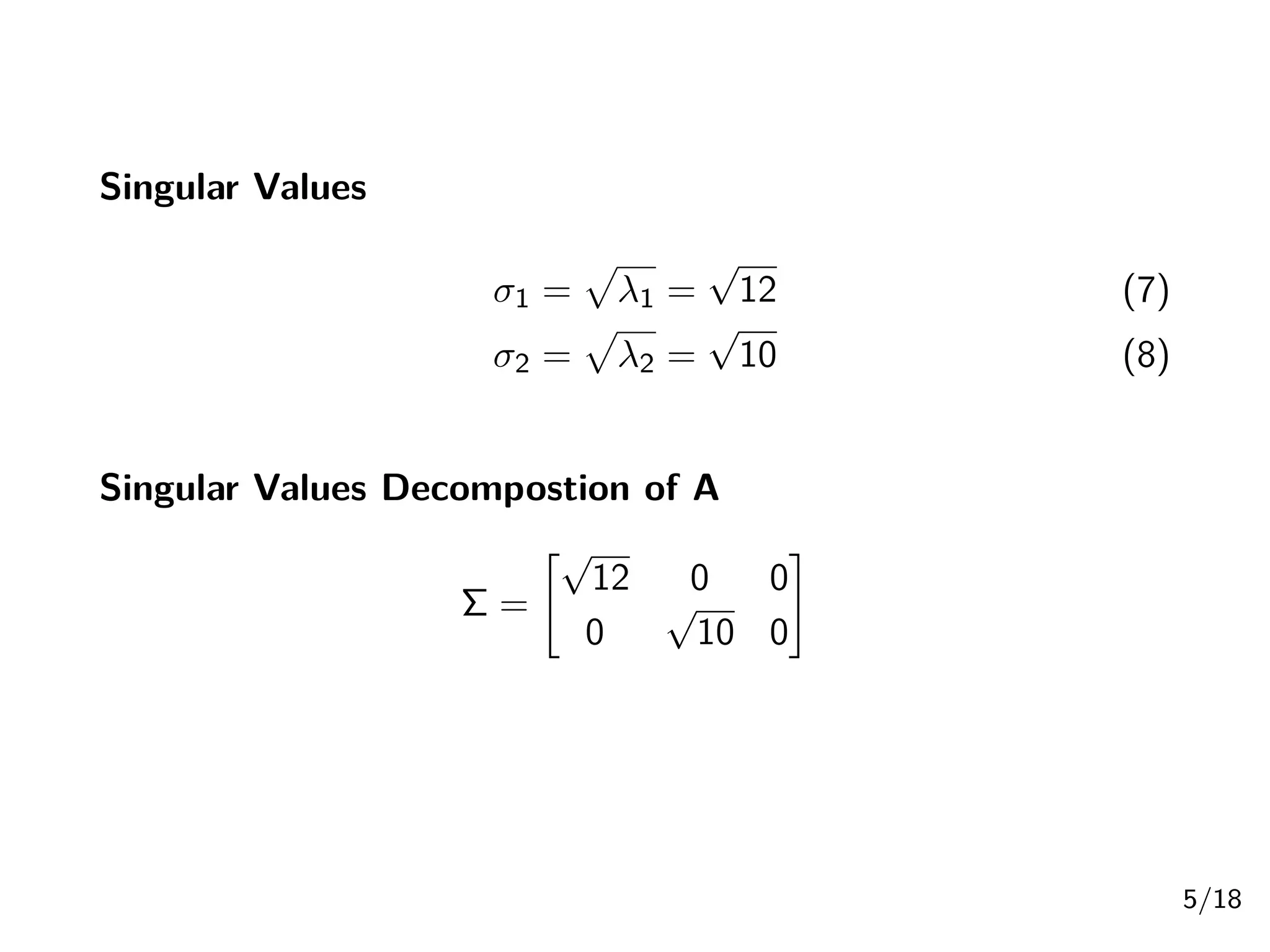
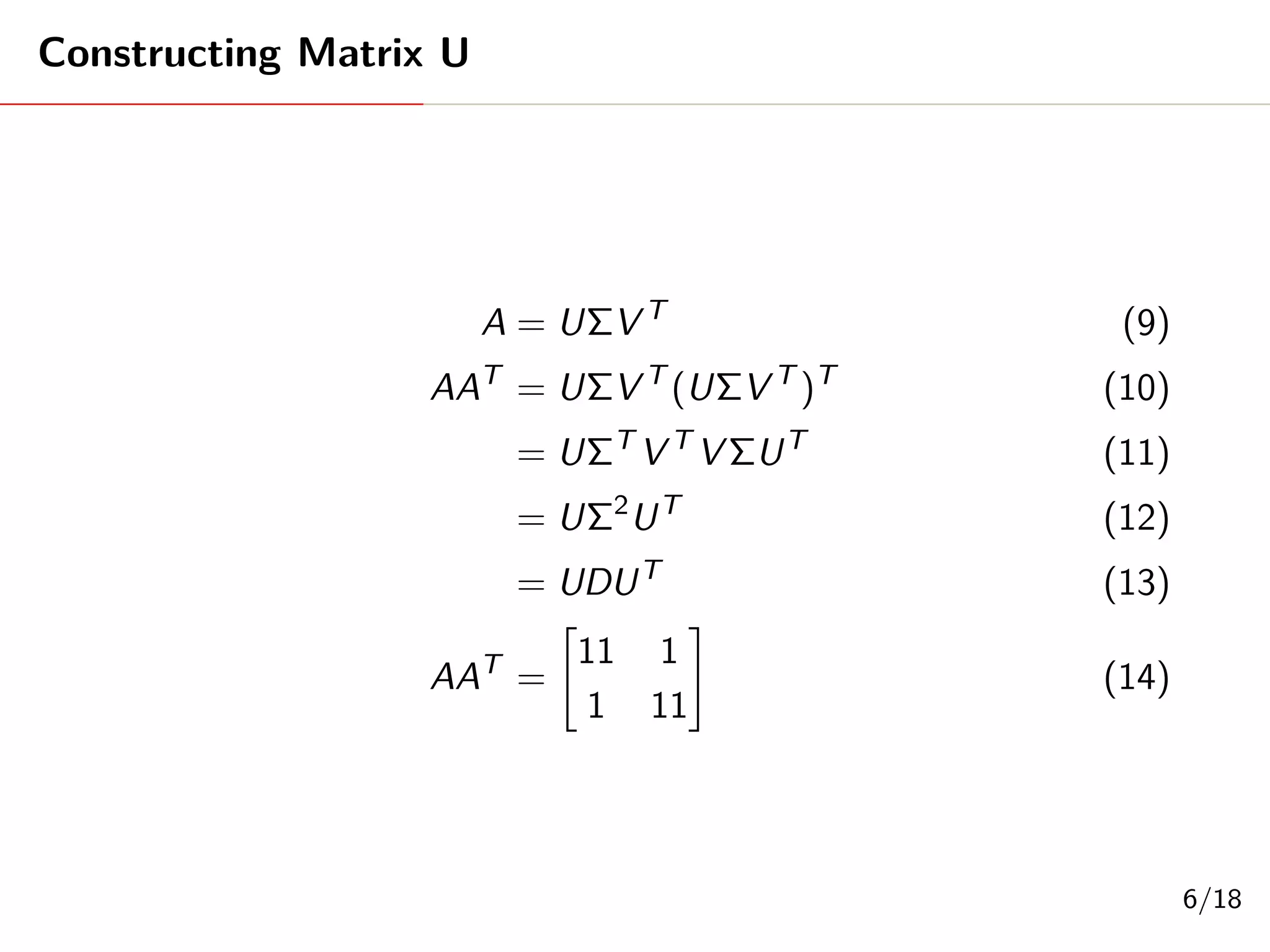
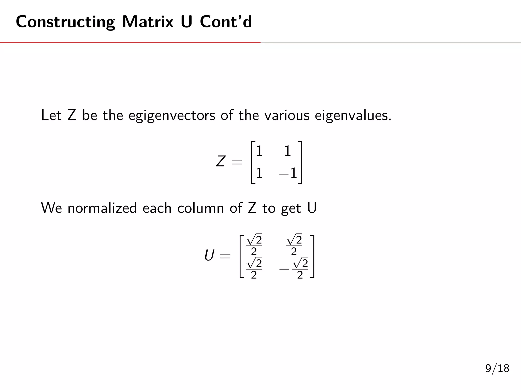
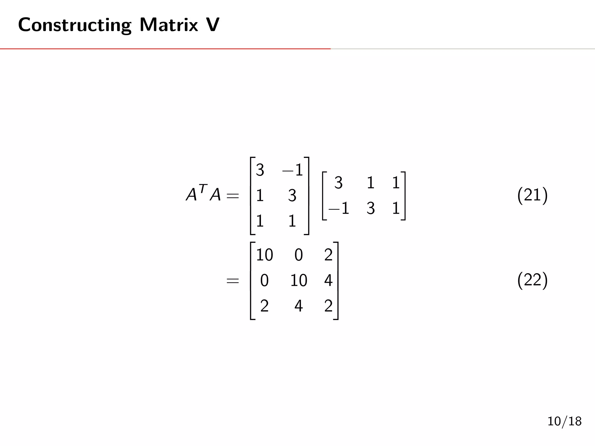
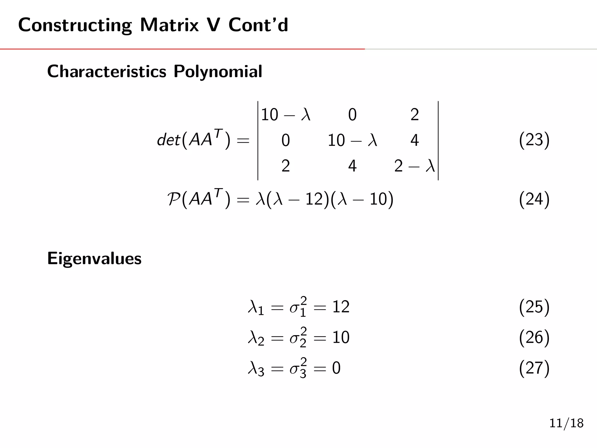
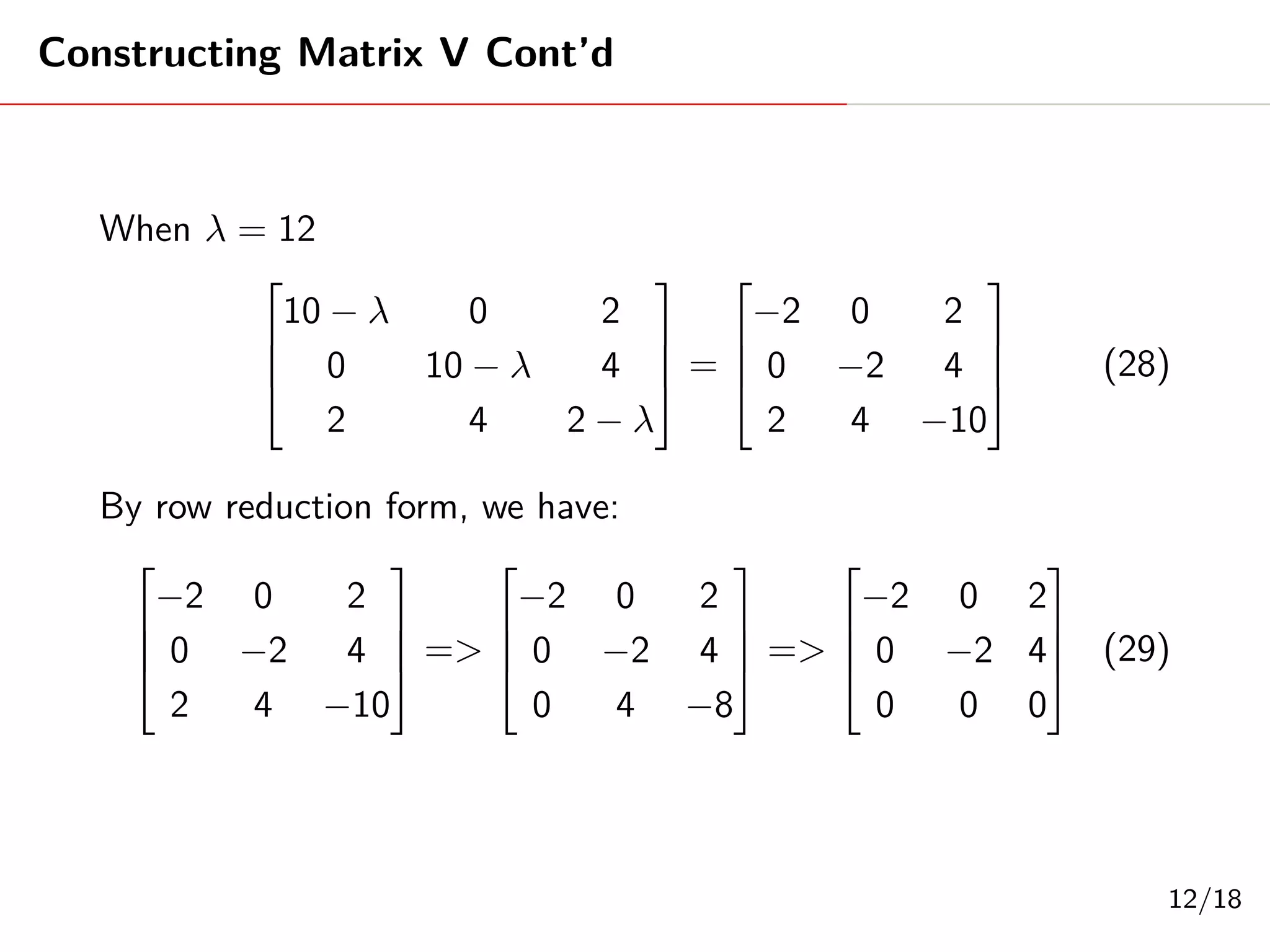
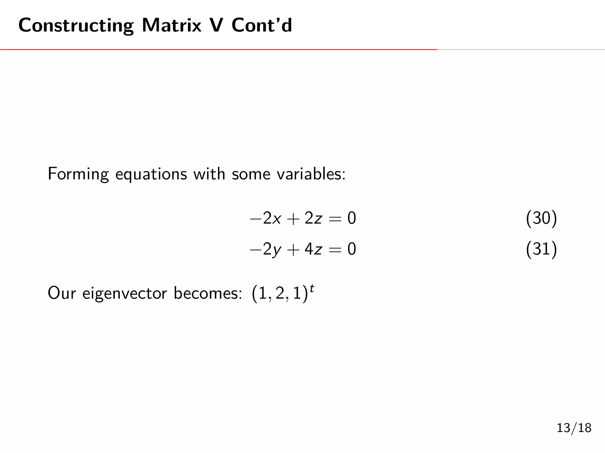
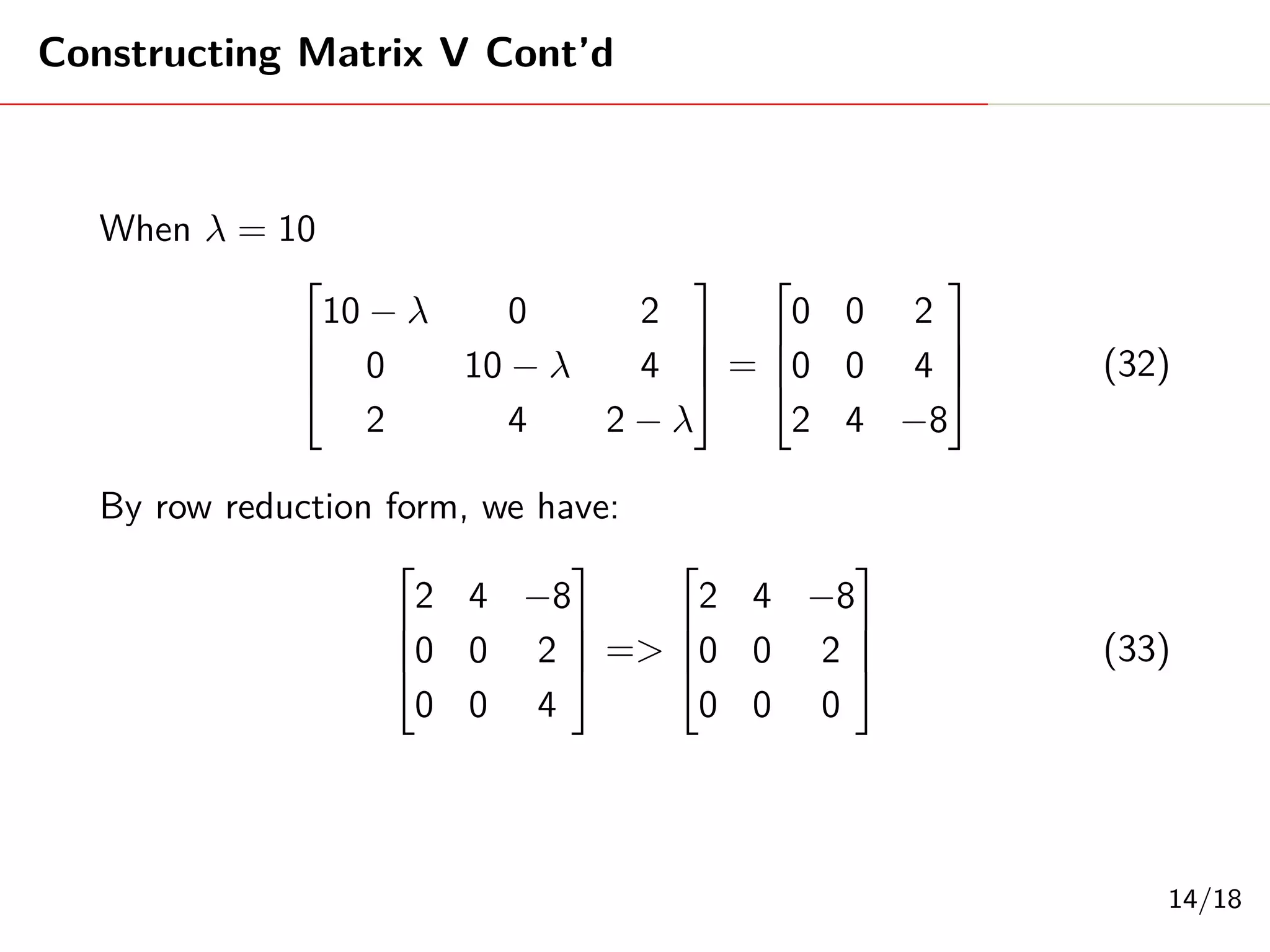
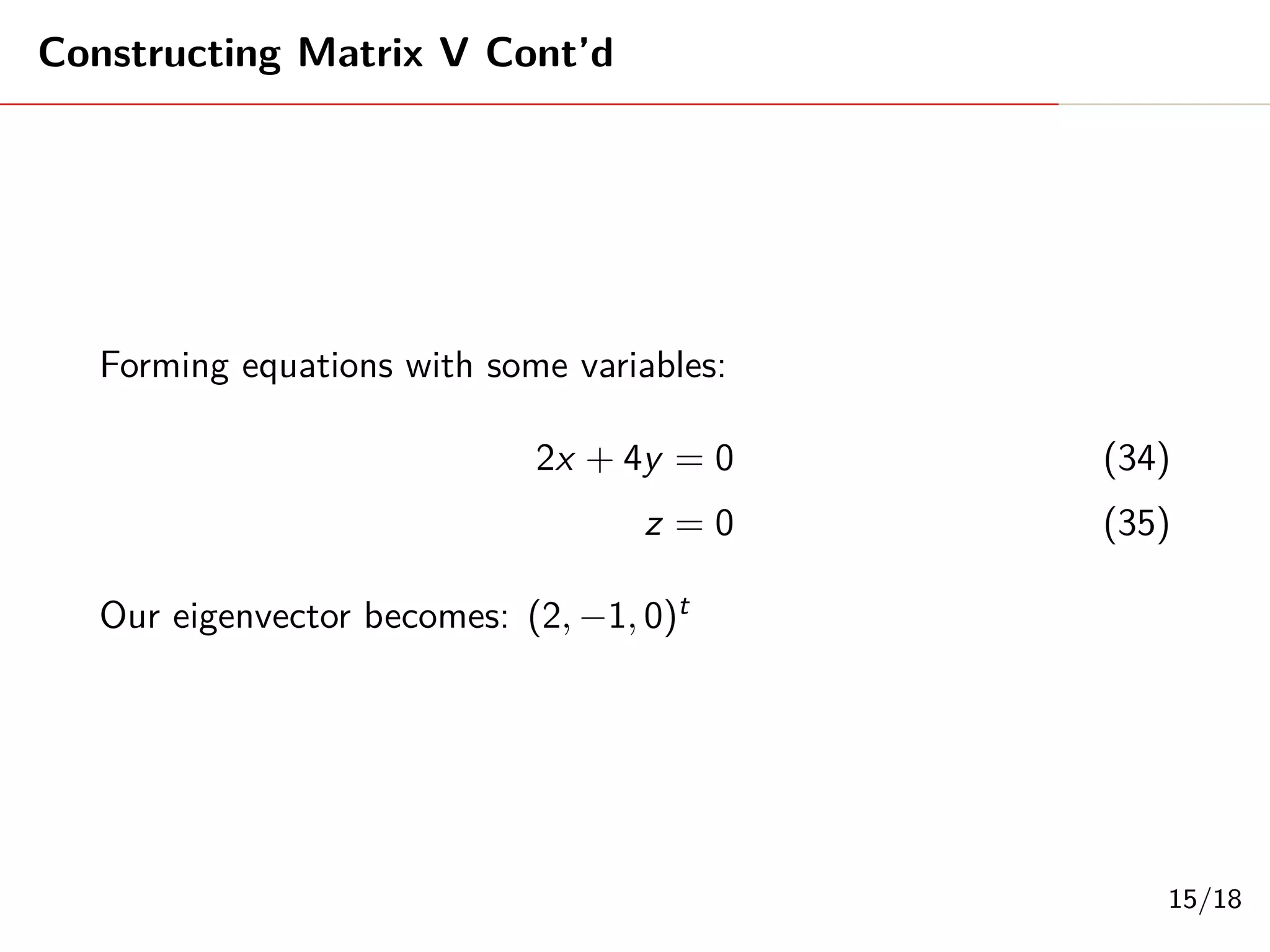
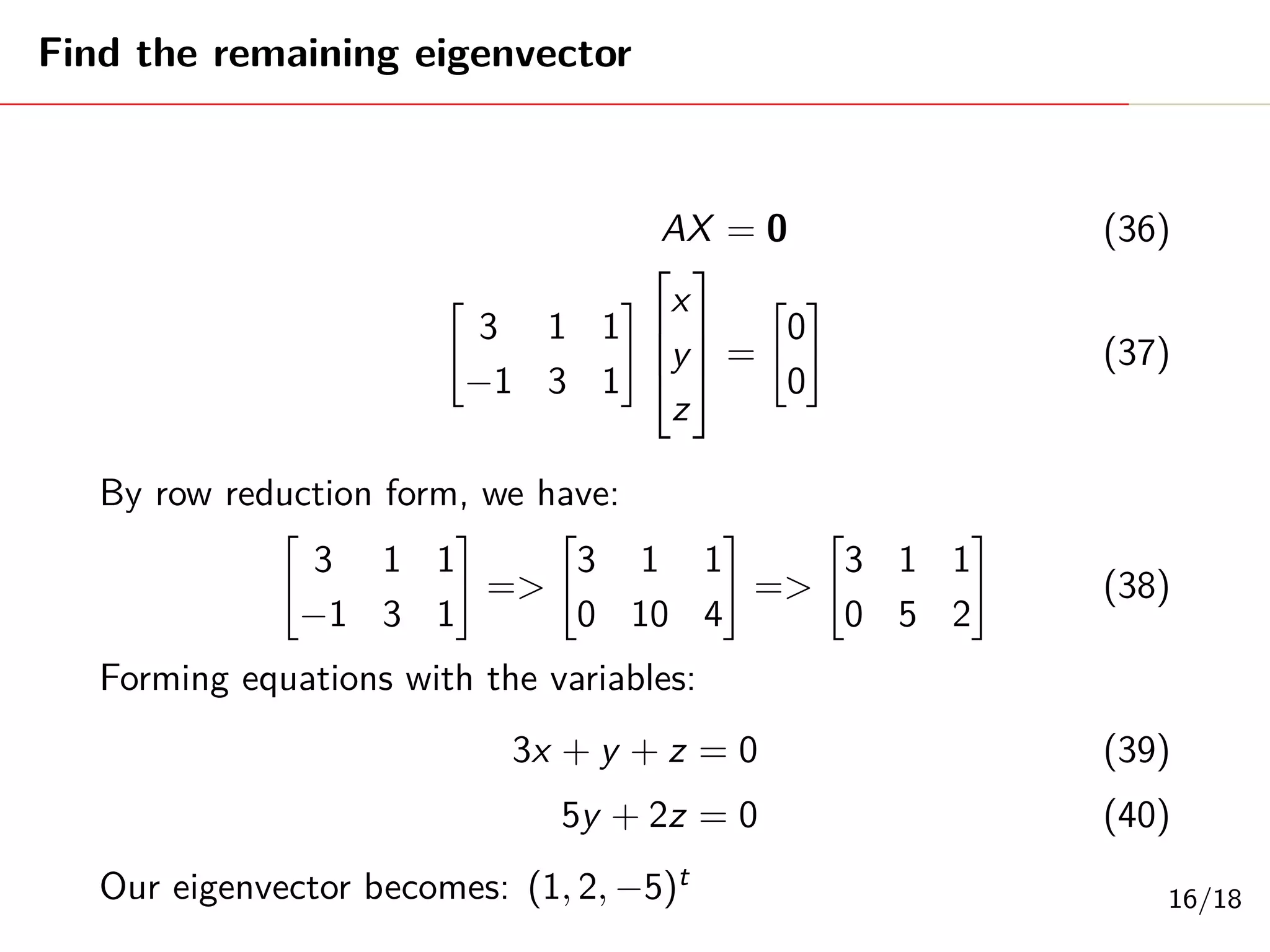
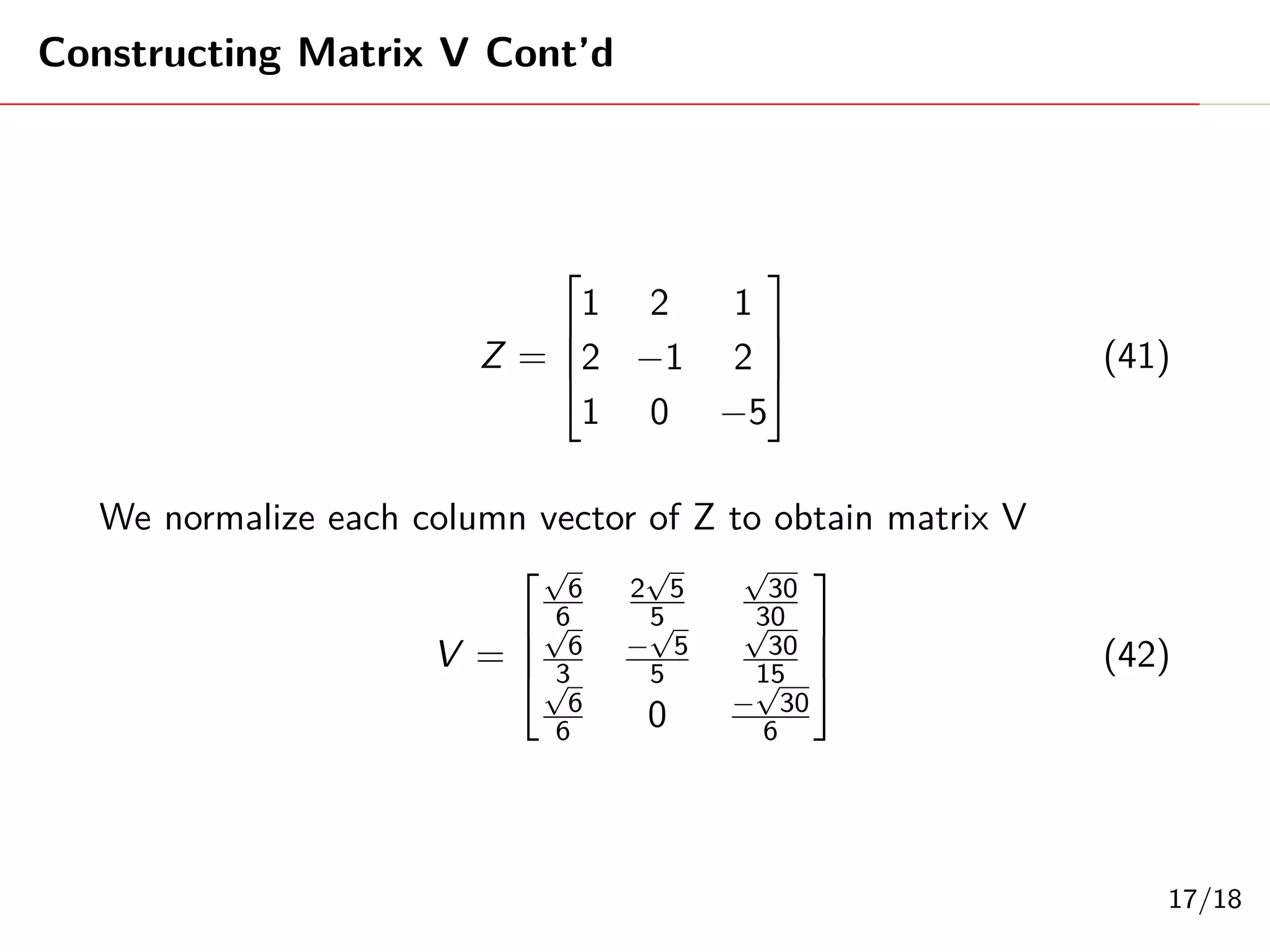
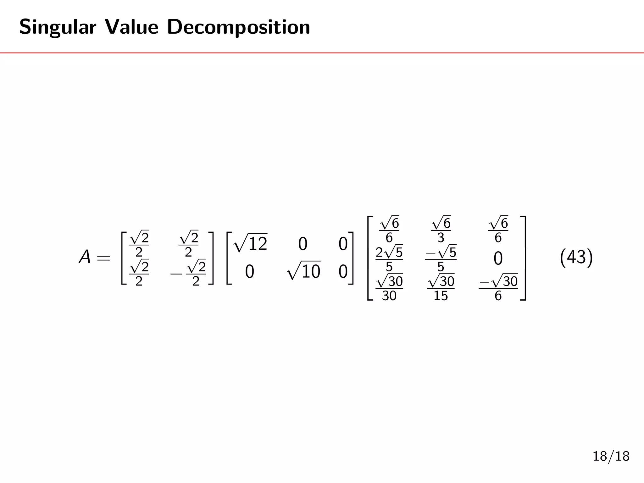
Singular Value Decomposition (SVD) decomposes a matrix A into three matrices: U, Σ, and V. The document provides an example of using SVD to decompose the matrix A = [[3, 1, 1], [-1, 3, 1]]. It finds the singular values and constructs the U, Σ, and V matrices. The SVD of A is written as A = UΣV^T, where U and V are orthogonal matrices and Σ is a diagonal matrix containing the singular values of A.

1. Singular Value Decomposition (SVD)
Isaac Amornortey Yowetu
December 31, 2021

2. Example 3
Find the matrices U Σ and V for the matrix
A =
"
3 1 1
−1 3 1
#
2/18

3. Finding the Singular Values
Solution
A =
"
3 1 1
−1 3 1
#
AT
=




3 −1
1 3
1 1




AAT
=
"
11 1
1 11
#
3/18

4. Characteristics Polynomial
det(AT
A) =

9. 11 − λ 1
1 11 − λ

14. (1)
P(AT
A) = (11 − λ)(11 − λ) − 1 (2)
= λ2
− 22λ + 120 (3)
= (λ − 12)(λ − 10) (4)
Eigenvalues
λ1 = σ2
1 = 12 (5)
λ2 = σ2
2 = 10 (6)
4/18

15. Singular Values
σ1 =
p
λ1 =
√
12 (7)
σ2 =
p
λ2 =
√
10 (8)
Singular Values Decompostion of A
Σ =
"√
12 0 0
0
√
10 0
#
5/18

16. Constructing Matrix U
A = UΣV T
(9)
AAT
= UΣV T
(UΣV T
)T
(10)
= UΣT
V T
V ΣUT
(11)
= UΣ2
UT
(12)
= UDUT
(13)
AAT
=
"
11 1
1 11
#
(14)
6/18

17. Constructing Matrix U Cont’d
When λ = 12
"
11 − λ 1
1 11 − λ
#
=
"
−1 1
1 −1
#
(15)
By row reduction form, we have:
"
−1 1
1 −1
#
=>
"
−1 1
0 0
#
(16)
Forming equations with some variables:
−x + y = 0 (17)
Our eigenvector becomes: (1, 1)t
7/18

18. Constructing Matrix U Cont’d
When λ = 10
"
11 − λ 1
1 11 − λ
#
=
"
1 1
1 1
#
(18)
By row reduction form, we have:
"
1 1
1 1
#
=>
"
1 1
0 0
#
(19)
Forming equations with some variables:
x + y = 0 (20)
Our eigenvector becomes: (1, −1)t
8/18

19. Constructing Matrix U Cont’d
Let Z be the egigenvectors of the various eigenvalues.
Z =
"
1 1
1 −1
#
We normalized each column of Z to get U
U =
"√
2
2
√
2
2
√
2
2 −
√
2
2
#
9/18

20. Constructing Matrix V
AT
A =




3 −1
1 3
1 1




"
3 1 1
−1 3 1
#
(21)
=




10 0 2
0 10 4
2 4 2



 (22)
10/18

21. Constructing Matrix V Cont’d
Characteristics Polynomial
det(AAT
) =

29. 10 − λ 0 2
0 10 − λ 4
2 4 2 − λ

37. (23)
P(AAT
) = λ(λ − 12)(λ − 10) (24)
Eigenvalues
λ1 = σ2
1 = 12 (25)
λ2 = σ2
2 = 10 (26)
λ3 = σ2
3 = 0 (27)
11/18

38. Constructing Matrix V Cont’d
When λ = 12




10 − λ 0 2
0 10 − λ 4
2 4 2 − λ



 =




−2 0 2
0 −2 4
2 4 −10



 (28)
By row reduction form, we have:




−2 0 2
0 −2 4
2 4 −10



 =>




−2 0 2
0 −2 4
0 4 −8



 =>




−2 0 2
0 −2 4
0 0 0



 (29)
12/18

39. Constructing Matrix V Cont’d
Forming equations with some variables:
−2x + 2z = 0 (30)
−2y + 4z = 0 (31)
Our eigenvector becomes: (1, 2, 1)t
13/18

40. Constructing Matrix V Cont’d
When λ = 10




10 − λ 0 2
0 10 − λ 4
2 4 2 − λ



 =




0 0 2
0 0 4
2 4 −8



 (32)
By row reduction form, we have:




2 4 −8
0 0 2
0 0 4



 =>




2 4 −8
0 0 2
0 0 0



 (33)
14/18

41. Constructing Matrix V Cont’d
Forming equations with some variables:
2x + 4y = 0 (34)
z = 0 (35)
Our eigenvector becomes: (2, −1, 0)t
15/18

42. Find the remaining eigenvector
AX = 0 (36)
"
3 1 1
−1 3 1
#




x
y
z



 =
"
0
0
#
(37)
By row reduction form, we have:
"
3 1 1
−1 3 1
#
=>
"
3 1 1
0 10 4
#
=>
"
3 1 1
0 5 2
#
(38)
Forming equations with the variables:
3x + y + z = 0 (39)
5y + 2z = 0 (40)
Our eigenvector becomes: (1, 2, −5)t
16/18

43. Constructing Matrix V Cont’d
Z =




1 2 1
2 −1 2
1 0 −5



 (41)
We normalize each column vector of Z to obtain matrix V
V =




√
6
6
2
√
5
5
√
30
30
√
6
3
−
√
5
5
√
30
15
√
6
6 0 −
√
30
6



 (42)
17/18

44. Singular Value Decomposition
A =
"√
2
2
√
2
2
√
2
2 −
√
2
2
# "√
12 0 0
0
√
10 0
#




√
6
6
√
6
3
√
6
6
2
√
5
5
−
√
5
5 0
√
30
30
√
30
15
−
√
30
6



 (43)
18/18