Download to read offline

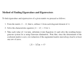
![Eigenvalue Problems
(Mathematical Background)
a11 λx1 a12x2 a1nxn 0
a21x1 a22 x2 a1nxn 0
an1x1 an2x2 ann xn 0
D Determinant AI
AX0
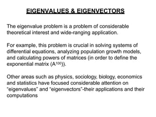
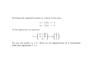
The roots of polynomial D(λ) are the eigenvalues of the eigen system
A solution {X} to [A]{X} = λ{X} is an eigen vector
(homogeneous system)
AIX0 (eigen system)
1 2 3
4 5 6
7 8 9
1-c 2 3
4 5-c 6
7 8 9-c](https://image.slidesharecdn.com/eigenvalueandeigenvector-221215041608-cc3c9d5c/85/Eigen-value-and-Eigen-Vector-pptx-4-320.jpg)
![15
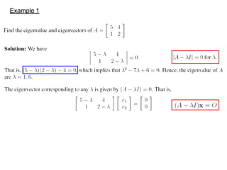
The Power Method
(An iterative approach for determining the largest eigenvalue)
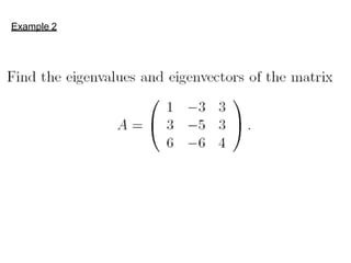
Example (3):
Iteration 1: initialization [x1, x2, x3]T = [1 1 1]T
Iteration 2: A [10 1]T
Iteration 3: A [1 -11]T
Iteration 4: A [-0.751 -0.75]T
Iteration 4: A [-0.7141 -0.714]T
(Exact solution = 6.070)](https://image.slidesharecdn.com/eigenvalueandeigenvector-221215041608-cc3c9d5c/85/Eigen-value-and-Eigen-Vector-pptx-17-320.jpg)
![21
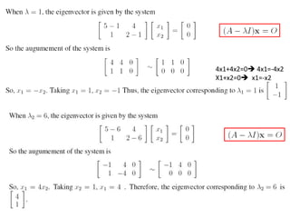
Power Method for Lowest Eigenvalue
(An iterative approach for determining the lowesteigenvalue)
0.141
0.141
0.281
0.562 0.281
0.281 0.422
0.422
A1
0.281
0.751
0.751
0.884
0.1411
0.281
0.562 0.2811 1.124 1.124 1
0.281 0.4221 0.884
0.281
0.141
0.422
Iteration 1:
Iteration 3:
Exact solution is 0.955 which is the reciprocal of the smallest eigenvalue,
1.0472 of [A].
Iteration 2:
0.715
0.715
0.984 1
0.984
0.281 0.1410.751 0.704
0.562 0.281 1
0.281 0.4220.751 0.704
0.141
0.281
0.422
0.709
0.709
0.964
1
0.964
0.1410.715 0.684
0.281
0.562 0.281
1
0.281 0.4220.715 0.684
0.141
0.281
0.422
Idea: The largest eigenvalue of [A]-1 is the reciprocal of the lowest
eigenvalue of [A]
1.7783.556
0 1.778
3.556 1.778 0
Example (5): A 1.778 0.281 3.556
0.422](https://image.slidesharecdn.com/eigenvalueandeigenvector-221215041608-cc3c9d5c/85/Eigen-value-and-Eigen-Vector-pptx-21-320.jpg)

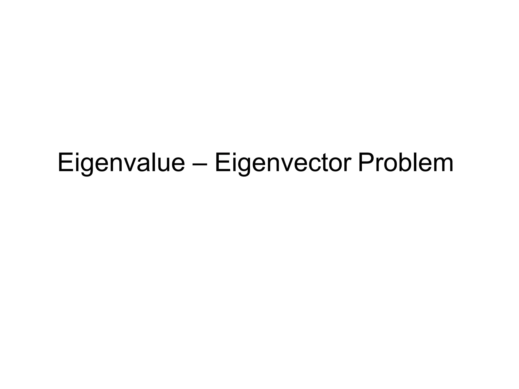
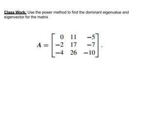
This document discusses the eigenvalue-eigenvector problem, which is important for solving differential equations, modeling population growth, and calculating matrix powers. It defines eigenvalues and eigenvectors and provides examples of solving eigenvalue problems. The power method, an iterative approach, is described for finding the dominant or lowest eigenvalue of a matrix. Solving eigenvalue problems has applications in many fields including physics, biology, economics and statistics.