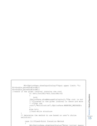
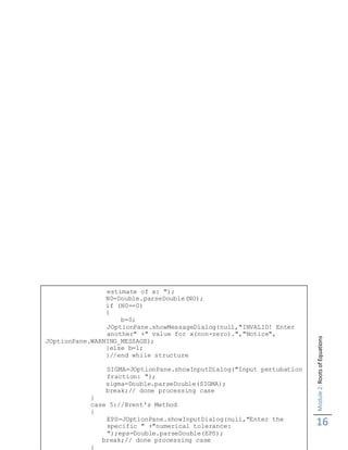
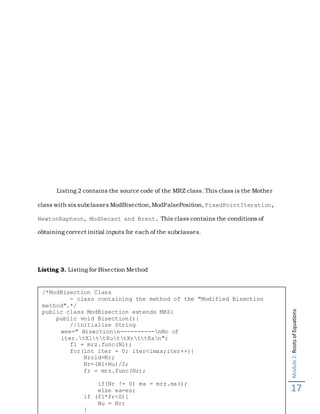
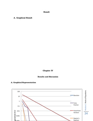
This document discusses various methods for finding the roots of equations, including bracketing methods like bisection and false position, open methods like fixed point iteration and Newton-Raphson, and the secant method. It provides formulas and explanations of how each method works to successively approximate a root through iterative calculations. Examples are given of applying the methods to solve engineering problems involving equations of state.

![Module2:RootsofEquations
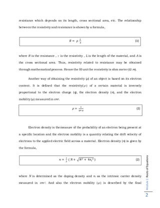
5
It comprises different methods which the roots may be found within the two
initial guesses which are typically changes the signs. The methods present here give
strategies which reducesthe width of the bracket until the root will be found.
Bisection Method
It is called the binary chopping or the Bolzano’s method. A Bracketing method
which finds root of a given continuous function over an interval 𝑥 𝑙 and𝑥 𝑢 such that
f(𝑥 𝑙) and f(𝑥 𝑢) will have an opposite signs that gives f(𝑥 𝑙) f(𝑥 𝑢) < 0. The method divides
the interval in two by computing the midpoint 𝑥 𝑟= (𝑥𝑙+𝑥 𝑢)/2 of the interval. Either f(𝑥 𝑙)
and f(𝑥 𝑟) or f(𝑥 𝑟) and f(𝑥 𝑢) will have opposite signs and it brackets a root, we must
select a subinterval within the interval and apply the same bisection step. There will
be a 50% of chance of getting a function equals to zero. If f(𝑥𝑙) f(𝑥 𝑟) < 0, then the
method sets equal 𝑥 𝑢 to𝑥 𝑟, and if f(𝑥 𝑢) f(𝑥 𝑟)< 0, then the method sets 𝑥 𝑙equal to 𝑥 𝑟. For
both cases, the new f(𝑥 𝑙) and f(𝑥 𝑢) will have opposite signs, so that the method is
applicable to this smaller interval.
The continuous function on the given interval [𝑥𝑙,𝑥 𝑢 ] and f(𝑥 𝑙) f(𝑥 𝑢) < 0 states
that the bisection converges to a root of the function and the true error is halved in
each step and the method converges linearly if f(𝑥 𝑙) and f(𝑥 𝑢) will have different signs.
This method gives only a range where the root exists and not the estimation where is
the roots location. The smallest bracket is where the root can be found. Its true error
of n steps can be solved by the equation;
𝜀 𝑡 =
𝑥 𝑙+𝑥 𝑢
2
(2.1)](https://image.slidesharecdn.com/83662164-case-study-1-150908145954-lva1-app6892/85/83662164-case-study-1-5-320.jpg)
![Module2:RootsofEquations
10
multiplicity higher than one it converges to that factor is a linear and quadratic factors
that have a small value which has real roots will tend to diverge to infinity. To find for
the zero of polynomial can be implemented with a programming language.
Müller's method
A root finding method that solves for the root of the form f(x) = 0 of the single variable x
and a scalar function whenever there’s no information about the derivatives that
exists. It’s the generalizes the secant method but it uses three points of quadratic
interpolation noted by as xk, xk-1 and xk-2.The The parabola going through the three
points (xk, f(xk)), (xk-1, f(xk-1)) and (xk-2, f(xk-2)) when
It can be written in the Newton form, where f[xk, xk-1] and f[xk, xk-1, xk-2] denote
divided differences;
where;
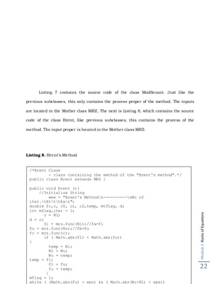
Brent’s Method](https://image.slidesharecdn.com/83662164-case-study-1-150908145954-lva1-app6892/85/83662164-case-study-1-10-320.jpg)