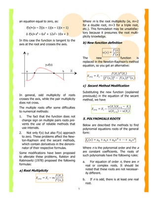
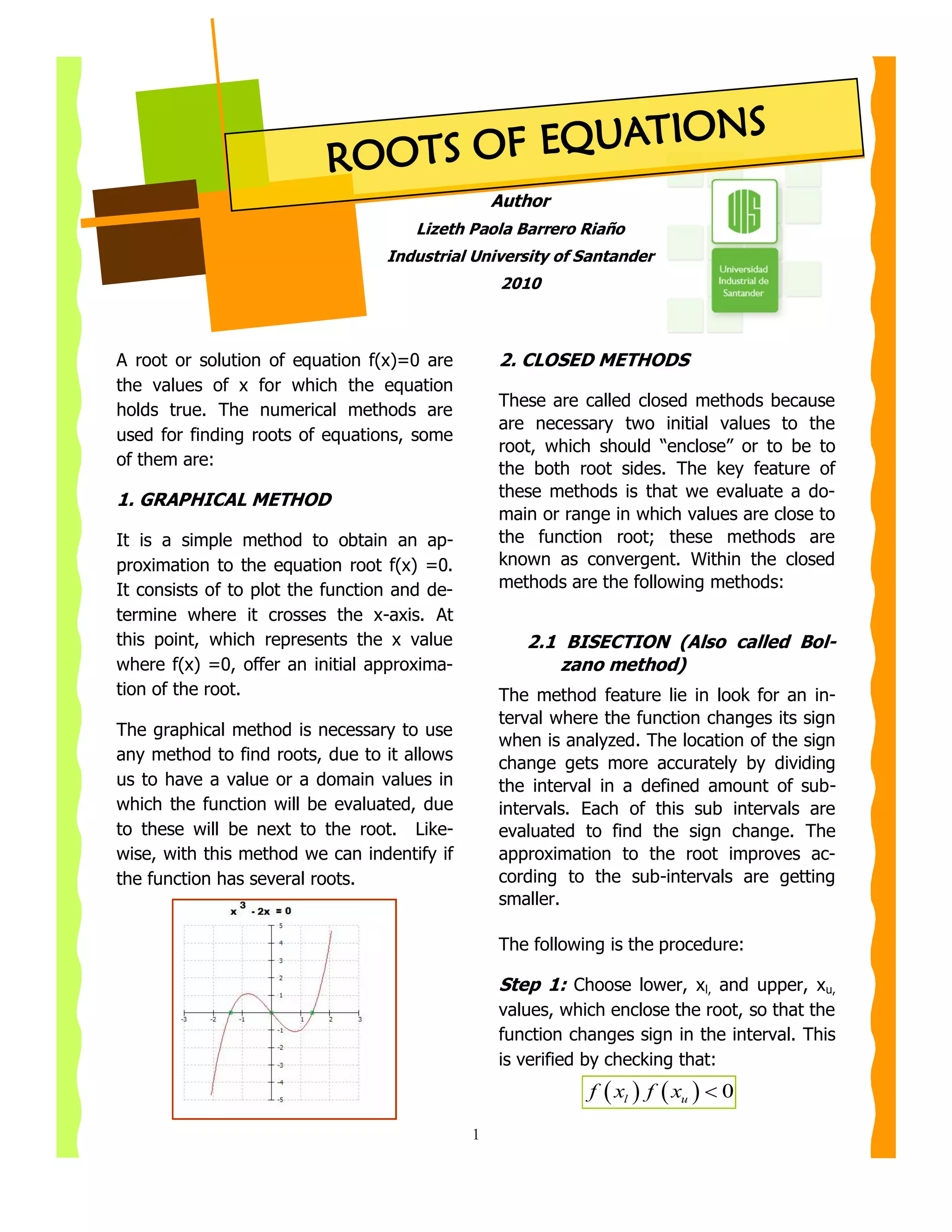
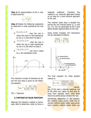
This document discusses numerical methods for finding roots or solutions of equations. Some key methods mentioned include: - Graphical method to obtain initial approximations of roots by plotting the function - Bisection method which divides intervals in half to find where the function changes sign - False position method which uses a straight line between two points to get a better approximation than bisection - Iteration methods like Newton-Raphson which use formulas to iteratively predict new values converging on the root - 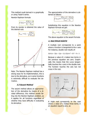Multiple roots can be found by modifying Newton-Raphson or using methods like Bairstow's which divides polynomials

1. ROOTS OF EQUATIONS
Author
Lizeth Paola Barrero Riaño
Industrial University of Santander
2010
A root or solution of equation f(x)=0 are 2. CLOSED METHODS
the values of x for which the equation
These are called closed methods because
holds true. The numerical methods are
are necessary two initial values to the
used for finding roots of equations, some
root, which should “enclose” or to be to
of them are: the both root sides. The key feature of
1. GRAPHICAL METHOD these methods is that we evaluate a do-
main or range in which values are close to
It is a simple method to obtain an ap- the function root; these methods are
proximation to the equation root f(x) =0. known as convergent. Within the closed
It consists of to plot the function and de- methods are the following methods:
termine where it crosses the x-axis. At
this point, which represents the x value 2.1 BISECTION (Also called Bol-
where f(x) =0, offer an initial approxima- zano method)
tion of the root. The method feature lie in look for an in-
terval where the function changes its sign
The graphical method is necessary to use
when is analyzed. The location of the sign
any method to find roots, due to it allows change gets more accurately by dividing
us to have a value or a domain values in the interval in a defined amount of sub-
which the function will be evaluated, due intervals. Each of this sub intervals are
to these will be next to the root. Like- evaluated to find the sign change. The
wise, with this method we can indentify if approximation to the root improves ac-
the function has several roots. cording to the sub-intervals are getting
smaller.
The following is the procedure:
Step 1: Choose lower, xl, and upper, xu,
values, which enclose the root, so that the
function changes sign in the interval. This
is verified by checking that:
f  xl  f  xu   0
1

2. Step 2: An approximation of the xr root, relatively inefficient. Therefore this
is determined by: method is an improved alternative based
on an idea for a more efficient approach
xl  xu to the root.
xr 
2
This method raises draw a straight line
Step 3: Realize the following evaluations joining the two interval points (x, y) and
to determine in what subinterval the root (x1, y1), the cut generated by the x-axis
is: allows greater approximation to the root.
f  xl  f  xr   0
If , then the root is Using similar triangles, the intersection
within the lower or left subinterval, can be calculated as follows:
so, do xu=xr and return to step 2.
f  xl  f  xr   0
If , then the root is
within the top or right subinterval,
so, do xl=xr and return to step 2.
f  xl  f  xr   0
If , the root is equal
to xr; the calculations ends.
The final equation for False position
The maximum number of iterations to ob- method is:
tain the root value is given by the follow-
ing equation:
The calcula-
tion of the root xr requires replacing one
of the other two values so that they al-
TOL = Tolerance ways have opposite signs, what leads
these two points always enclose the root.
2.2 METHOD OF FALSE POSITION Sometimes, depending on the function,
this method works poorly, while the bi-
Although the bisection method is techni- section method leads better approxima-
cally valid to determine roots its focus is
tions. section method leads better ap-
2

3. section method leads better approxima- cate the root of f(x) = e-x – x
tions. Solution: Like f(x)=0 ó e-x – x=0
3. OPEN METHODS Expressing of the form x=g(x) result us:
x= e-x
These methods are based on formulas Beginning with an initial value of xo=0, we
that require a single initial value x, or a can apply the iterative equation xi+1=g(xi)
couple of them but do not necessarily that and calculate:
contain the root. Because of this feature,
sometimes these methods diverge or
move away from the root, according to i xi Ea(%) Et(%)
grows the number of iterations. It is im- 0 0 100.0
portant to know that when the open 1 1.000000 100.0 76.3
methods converge, these are more effi- 2 0.367879 171.8 35.1
cient than methods that use intervals. 3 0.692201 46.9 22.1
Open methods are: 4 0.500473 38.3 11.8
5 0.606244 17.4 6.89
3.1 SIMPLE FIXED POINT ITE-
RATION 6 0.545396 11.2 3.83
7 0.579612 5.90 2.20
Open methods employ a formula that pre-
8 0.560115 3.48 1.24
dicts the root, this formula can be devel-
oped for a single iteration of a fixed point 9 0.571143 1.93 0.705
(also called point iteration or successive 10 0.564879 1.11 0.399
substitution) to change the equation f (x)
= 0 so that is:
Thus, each iteration bring near increas-
x=g(x) ingly to the estimated value with the true
This formula is employ to predict a new x value of the root, that is to say
value in function of the previous x valor, 0.56714329
through:
3.2 NEWTON RAPHSON
xi+1=g(xi) METHOD
Subsequently, these iterations are used to The most widely used formula to find
calculate the approximate error so that roots, is the Newton Raphson, argues that
the least error indicates the root of the if it indicates the initial value of x1 as the
function in matter. value of the root, then it is possible to ex-
xi 1  xi tend a tangent line from the point (x1,f
a= x100 (x1)). Where this straight line crosses the
xi 1
x-axis will be the point of improve ap-
proach.
For instance:
Use simple iteration of a fixed point to lo-
3

4. This method could derived in a graphically The approximation of the derivative is ob-
or using Taylor’s series. tained as follows:
Newton Raphson formula
Substituting this equation in the Newton
From its reorder is obtained the value of Raphson formula we get:
the desired root.
The above equation is the secant formula.
4. MULTIPLES ROOTS
A multiple root corresponds to a point
where a function is tangential to the x axis
For instance, double root results of:
f(x)=(x – 3)(x – 1)(x – 1) ó f(x)=x3 – 5x2 – 7x - 3
Because a value of x makes two terms in
the previous equation are zero. Graphi-
cally this means that the curve tangen-
tially touches the x axis in the double root.
The function touches the axis but not
cross in the root.
Note: The Newton Raphson method has a
strong issue for its implementation, this is
due to the derivative, as in some functions
is extremely difficult to evaluate the de-
rivative.
3.3 Secant Method
The secant method allows an approxima-
tion of the derivative by means of a di-
vided difference; this method avoids fal-
ling into the Newton Raphson problem, as
it applies for all functions regardless of
whether they have difficulty in evaluating A triple root corresponds to the case
its derivative. where a value of x makes three terms in
an equation equal to zero, as:
4

5. an equation equal to zero, as: Where m is the root multiplicity (ie, m=2
for a double root, m=3 for a triple root,
f(x)=(x – 3)(x – 1)(x – 1)(x – 1) etc.). This formulation may be unsatisfac-
ó f(x)=x4 – 6x3 + 12x2– 10x + 3 tory because it presumes the root multi-
plicity knowledge.
In this case the function is tangent to the
axis at the root and crosses the axis. b) New function definition
The new function is
replaced in the Newton-Raphson’s method
equation, so you get an alternative:
c) Secant Method Modification
Substituting the new function (explained
In general, odd multiplicity of roots previously) in the equation of the secant
crosses the axis, while the pair multiplicity method, we have
does not cross.
The multiple roots offer some difficulties
to numerical methods:
1. The fact that the function does not
change sign on multiple pairs roots pre- 5. POLYNOMIALS ROOTS
vents the use of reliable methods that Below are described the methods to find
use intervals. polynomial equations roots of the general
2. Not only f(x) but also f'(x) approach form:
to zero. These problems affect the New-
ton-Raphson and the secant methods,
which contain derivatives in the denomi-
nator of their respective formulas. Where n is the polynomial order and the a
Some modifications have been proposed are constant coefficients. The roots of
to alleviate these problems, Ralston and such polynomials have the following rules:
Rabinowitz (1978) proposed the following a. For equation of order n, there are n
formulas: real or complex roots. It should be
a) Root Multiplicity noted that these roots are not necessar-
ily different.
b. If n is odd, there is at least one real
root.
5

6. c. If the roots are complex, there is a Thus, this parable is used to intersect the
conjugate pair (i.e., λ + µi y λ - µi) where three points [x0, f(x0)], [x1, f(x1)] and [x2, f
(x2)]. The coefficients of the previous equa-
tion are evaluated by substituting one of
these three points to make:
A predecessor of Muller method is the se-
cant method, which obtain root, estimating f ( x0 )  a( x0  x2 )2  b( x0  x2 )  c
a projection of a straight line on the x-axis
through two function values (Shape f ( x1 )  a( x1  x2 ) 2  b( x1  x2 )  c
1). Muller's method takes a similar view, but
f ( x2 )  a( x2  x2 ) 2  b( x2  x2 )  c
projected a parabola through three points
(Shape 2).
f ( x2 )  c
The last equation generated that ,
The method consist in to obtain the coeffi- in this way, we can have a system of two
cients of the three points, replace them in equations with two unknowns:
the quadratic formula and get the point
where the parabola intersects the x-axis The f ( x0 )  f ( x2 )  a( x0  x2 )2  b( x0  x2 )
approach is easy to write, as appropriate
this would be: f ( x1 )  f ( x2 )  a( x1  x2 ) 2  b( x1  x2 )
f 2 ( x)  a( x  x2 ) 2  b( x  x2 )  c Defining this way:
h0  x1  x0 h1  x2  x1
f ( x 2 )  f ( x1 ) f ( x1 )  f ( x 2 )
1  0 
x 2  x1 x1  x0
Substituting in the system:
(h0  h1 )b  (h0  h1 ) 2 a  h0 0  h1 1
h1b  h1 a  h1 1
2
The coefficients are:
Shape 1 1   0
a b  ah1   1
h1  h0
c  f ( x2 )
Finding the root, the conventional solution is
implemented, but due to rounding error po-
tential, we use an alternative formulation:
 2c
x3  x 2 
b  b 2  4ac
Shape 2
6

7. Solving: use the synthetic division. So given
 2c
x3  x 2  fn(x) = anxn + an-1xn-1 + … + a2x2 + a1x + a0
b  b  4ac
2
By dividing between f2(x) = x2 – rx – s, we
The great advantage of this method is that have as a result the following polynomial
we find real and imaginary roots.
Finding the error this will be: fn-2(x) = bnxn-2 + bn-1xn-3 + … + b3x + b2
x3  x 2
Ea   100% with a residue R = b1(x-r) + b0, the residue
x3
will be zero only if b1 and b0 are.
To be an approximation method, this is per-
formed sequentially and iteratively, where The terms b and c, are calculated using the
x1, x2, x3replace the points x0, x1, x2 carrying following recurrence relation:
the error to a value close to zero.
bn = an
5. 1 Bairstow’s Method bn-1 = an-1 + rbn
bi = ai + rbi+1 + sbi+2
Bairstow's method is an iterative process
related approximately with Muller and New- cn = bn
ton-Raphson methods. The mathematical cn-1 = bn-1 + rcn
process depends of dividing the polynomial ci = bi + rci+1 + sci+2
between a factor.
Finally, the approximate error in r and s can
Given a polynomial fn(x) find two factors, a
be estimated as:
quadratic polynomial f2(x) = x2 – rx – s y fn-2
(x). The general procedure for the Bairstow
method is:
1. Given fn(x) y r0 y s0 When both estimated errors failed, the roots
2. Using Newton-Raphson method calcu- values can be determined as:
late f2(x) = x2 – r0x – s0 y fn-2(x), such as,
the residue of fn(x)/ f2(x) be equal to zero.
3. The roots f2(x) are determined, using
the general formula.
4. Calculate fn-2(x)= fn(x)/ f2(x). BIBLIOGRAPHY
5. Do fn(x)= fn-2(x)
6. If the polynomial degree is greater CHAPRA, Steven C. y CANALE, Raymond P.:
than three, back to step 2 Métodos Numéricos para Ingenieros.
7. If not, we finish McGraw Hill 2007. 5th edition.
The main difference of this method in rela- http://numerical-methods.com/roots.htm
tion to others, allows calculating all the poly-
nomial roots (real and imaginaries).
To calculate the polynomials division, we
7