This document describes using the Gauss-Seidel method to solve a system of quadratic equations to estimate the amount of nickel in the organic phase of a liquid-liquid extraction process given experimental data. Initially, the method converges slowly with errors over 50%. Rearranging the equations to make the coefficient matrix more diagonally dominant improves convergence, with errors dropping below 5% after 6 iterations.

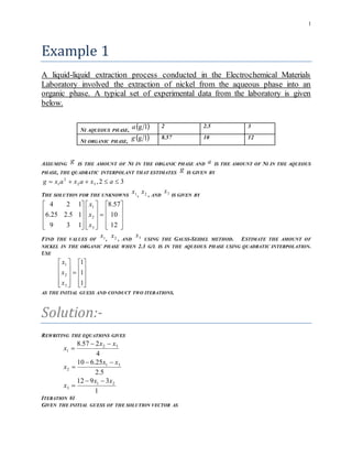
1. 1
Example 1
A liquid-liquid extraction process conducted in the Electrochemical Materials
Laboratory involved the extraction of nickel from the aqueous phase into an
organic phase. A typical set of experimental data from the laboratory is given
below.
NI AQUEOUS PHASE,
 lga 2 2.5 3
NI ORGANIC PHASE,
 lgg 8.57 10 12
ASSUMING
g IS THE AMOUNT OF NI IN THE ORGANIC PHASE AND a IS THE AMOUNT OF NI IN THE AQUEOUS
PHASE, THE QUADRATIC INTERPOLANT THAT ESTIMATES
g IS GIVEN BY
32,32
2
1  axaxaxg
THE SOLUTION FOR THE UNKNOWNS 1x , 2x , AND 3x
IS GIVEN BY































12
10
57.8
139
15.225.6
124
3
2
1
x
x
x
FIND THE VALUES OF 1x , 2x , AND 3x
USING THE GAUSS-SEIDEL METHOD. ESTIMATE THE AMOUNT OF
NICKEL IN THE ORGANIC PHASE WHEN 2.3 G/L IS IN THE AQUEOUS PHASE USING QUADRATIC INTERPOLATION.
USE





















1
1
1
3
2
1
x
x
x
AS THE INITIAL GUESS AND CONDUCT TWO ITERATIONS.
Solution:-
REWRITING THE EQUATIONS GIVES
4
257.8 32
1
xx
x


5.2
25.610 31
2
xx
x


1
3912 21
3
xx
x


ITERATION #1
GIVEN THE INITIAL GUESS OF THE SOLUTION VECTOR AS

2. 2





















1
1
1
3
2
1
x
x
x
WE GET
4
11257.8
1

x
3925.1
5.2
13925.125.610
2

x
11875.0
1
11875.033925.1912
3

x
88875.0
THE ABSOLUTE RELATIVE APPROXIMATE ERROR FOR EACH ix
THEN IS
100
3925.1
13925.1
1


a
%187.28
100
11875.0
111875.0
2


a
%11.742
100
88875.0
188875.0
3



a
%52.212
AT THE END OF THE FIRST ITERATION, THE ESTIMATE OF THE SOLUTION VECTOR IS






















88875.0
11875.0
3925.1
3
2
1
x
x
x
AND THE MAXIMUM ABSOLUTE RELATIVE APPROXIMATE ERROR IS %11.742 .
ITERATION #2
THE ESTIMATE OF THE SOLUTION VECTOR AT THE END OF ITERATION #1 IS






















88875.0
11875.0
3925.1
3
2
1
x
x
x
NOW WE GET
4
)88875.0(11875.0257.8
1

x
3053.2
 
5.2
88875.03053.225.610
2

x
4078.1

3. 3
 
1
4078.133053.2912
3

x
5245.4
THE ABSOLUTE RELATIVE APPROXIMATE ERROR FOR EACH ix
THEN IS
100
3053.2
3925.13053.2
1


a
%596.39
100
4078.1
11875.04078.1
2



a
%44.108
100
5245.4
)88875.0(5245.4
3



a
%357.80
AT THE END OF THE SECOND ITERATION, THE ESTIMATE OF THE SOLUTION VECTOR IS






















5245.4
4078.1
3053.2
3
2
1
x
x
x
AND THE MAXIMUM ABSOLUTE RELATIVE APPROXIMATE ERROR IS %44.108 .
CONDUCTING MORE ITERATIONS GIVES THE FOLLOWING VALUES FOR THE SOLUTION VECTOR AND THE
CORRESPONDING ABSOLUTE RELATIVE APPROXIMATE ERRORS.
ITERATION
1x %1a 2x %2a 3x %3a
1
2
3
4
5
6
1.3925
2.3053
3.9775
7.0584
12.752
23.291
28.1867
39.5960
42.041
43.649
44.649
45.249
0.11875
–1.4078
–4.1340
–9.0877
–18.175
–34.930
742.1053
108.4353
65.946
54.510
49.999
47.967
–0.88875
–4.5245
–11.396
–24.262
–48.243
–92.827
212.52
80.357
60.296
53.032
49.708
48.030
AFTER SIX ITERATIONS, THE ABSOLUTE RELATIVE APPROXIMATE ERRORS ARE NOT DECREASING MUCH. IN
FACT, CONDUCTING MORE ITERATIONS REVEALS THAT THE ABSOLUTE RELATIVE APPROXIMATE ERROR
CONVERGES TO A VALUE OF %070.46 FOR ALL THREE VALUES WITH THE SOLUTION VECTOR DIVERGING
FROM THE EXACT SOLUTION DRASTICALLY.
ITERATION 1x %1a 2x %2a 3x %3a
32 8
101428.2  0703.46 8
103920.3  0703.46 8
101095.9  0703.46
THE EXACT SOLUTION VECTOR IS





















55.8
27.2
14.1
3
2
1
x
x
x

4. 4
TO CORRECT THIS, THE COEFFICIENT MATRIX NEEDS TO BE MORE DIAGONALLY DOMINANT. TO ACHIEVE A
MORE DIAGONALLY DOMINANT COEFFICIENT MATRIX, REARRANGE THE SYSTEM OF EQUATIONS BY
EXCHANGING EQUATIONS ONE AND THREE.































57.8
10
12
124
15.225.6
139
3
2
1
x
x
x
ITERATION #1
GIVEN THE INITIAL GUESS OF THE SOLUTION VECTOR AS





















1
1
1
3
2
1
x
x
x
WE GET
9
11312
1

x
88889.0
5.2
188889.025.610
2

x
3778.1
1
3778.1288889.0457.8
3

x
2589.2
THE ABSOLUTE RELATIVE APPROXIMATE ERROR FOR EACH ix
THEN IS
100
88889.0
188889.0
1


a
%5.12
100
3778.1
13778.1
2


a
%419.27
100
2589.2
12589.2
3


a
%730.55
AT THE END OF THE FIRST ITERATION, THE ESTIMATE OF THE SOLUTION VECTOR IS





















2589.2
3778.1
88889.0
3
2
1
x
x
x
and the maximum absolute relative approximate error is %730.55 .
ITERATION #2
THE ESTIMATE OF THE SOLUTION VECTOR AT THE END OF ITERATION #1 IS

5. 5





















2589.2
3778.1
88889.0
3
2
1
x
x
x
NOW WE GET
9
2589.213778.1312
1

x
62309.0
5.2
2589.2162309.025.610
2

x
5387.1
1
5387.1262309.0457.8
3

x
0002.3
THE ABSOLUTE RELATIVE APPROXIMATE ERROR FOR EACH ix
THEN IS
100
62309.0
88889.062309.0
1


a
%659.42
100
5387.1
3778.15387.1
2


a
%460.10
100
0002.3
2589.20002.3
3


a
%709.24
AT THE END OF THE SECOND ITERATION, THE ESTIMATE OF THE SOLUTION IS





















0002.3
5387.1
62309.0
3
2
1
x
x
x
AND THE MAXIMUM ABSOLUTE RELATIVE APPROXIMATE ERROR IS %659.42 .
CONDUCTING MORE ITERATIONS GIVES THE FOLLOWING VALUES FOR THE SOLUTION VECTOR AND THE
CORRESPONDING ABSOLUTE RELATIVE APPROXIMATE ERRORS.
ITERATION 1x %1a 2x %2a 3x %3a
1
2
3
4
5
6
0.88889
0.62309
0.48707
0.42178
0.39494
0.38890
12.5
42.659
27.926
15.479
6.7960
1.5521
1.3778
1.5387
1.5822
1.5627
1.5096
1.4393
27.419
10.456
2.7506
1.2537
3.5131
4.8828
2.2589
3.0002
3.4572
3.7576
3.9710
4.1357
55.730
24.709
13.220
7.9928
5.3747
3.9826

6. 6
AFTER SIX ITERATIONS, THE ABSOLUTE RELATIVE APPROXIMATE ERRORS SEEM TO BE DECREASING.
CONDUCTING MORE ITERATIONS ALLOWS THE ABSOLUTE RELATIVE APPROXIMATE ERROR DECREASE TO AN
ACCEPTABLE LEVEL.
ITERATION 1x %1a 2x %2a 3x %3a
199
200
1.1335
1.1337
0.014412
0.014056
–2.2389
–2.2397
0.034871
0.034005
8.5139
8.5148
0.010666
0.010403
THIS IS CLOSE TO THE EXACT SOLUTION VECTOR OF





















55.8
27.2
14.1
3
2
1
x
x
x
THE POLYNOMIAL THAT PASSES THROUGH THE THREE DATA POINTS IS THEN
      32
2
1 xaxaxag 
     5148.82397.21337.1
2
 aa
WHERE
g IS THE AMOUNT OF NICKEL IN THE ORGANIC PHASE AND a IS THE AMOUNT OF NICKEL IN THE
AQUEOUS PHASE.
WHEN
l3.2 g IS IN THE AQUEOUS PHASE, USING QUADRATIC INTERPOLATION, THE ESTIMATED AMOUNT OF
NICKEL IN THE ORGANIC PHASE IS
        5148.83.22397.23.21337.13.2
2
g
lg3608.9

7. 7
Example 2
A trunnion has to be cooled before it is shrink fitted into a steel hub.
Figure 1 Trunnion to be slid through the hub after contracting
.
The equation that gives the temperature fT
to which the trunnion has to be cooled
to obtain the desired contraction is given by
01088318.01074363.01038292.01050598.0)( 2427310
 
TTTTf ffff
Use
the bisection method of finding roots of equations to find the temperature fT
to
which the trunnion has to be cooled. Conduct three iterations to estimate the root
of the above equation. Find the absolute relative approximate error at the end of
each iteration and the number of significant digits at least correct at the end of
each iteration.
Solution:-
FROM THE DESIGNER’S RECORDS FOR THE PREVIOUS BRIDGE, THE TEMPERATURE TO WHICH THE TRUNNION
WAS COOLED WAS
F108 . HENCE ASSUMING THE TEMPERATURE TO BE BETWEEN
F100 AND
F150 , WE HAVE
F150, fT
,
F100, ufT
CHECK IF THE FUNCTION CHANGES SIGN BETWEEN
,fT
AND
ufT ,
.
   
24
27310
,
1088318.0)150(1074363.0
)150(1038292.0)150(1050598.0
150




 fTf f 
3
102903.1 

 
24
27310
,
1088318.0)100(1074363.0
)100(1038292.0)100(1050598.0
)100(




 fTf uf

8. 8
3
108290.1 

HENCE
           0108290.1102903.1100150 33
,,  
ffTfTf uff 
SO THERE IS AT LEAST ONE ROOT BETWEEN ,fT
AND ufT ,
THAT IS BETWEEN
150 AND
100 .
ITERATION 1
THE ESTIMATE OF THE ROOT IS
2
,,
,
uff
mf
TT
T



2
)100(150 

125
   
24
27310
,
1088318.0)125(1074363.0
)125(1038292.0)125(1050598.0
125




 fTf mf
4
102.3356 

           0103356.2102903.1125150 43
,,  
ffTfTf mff 
HENCE THE ROOT IS BRACKETED BETWEEN
,fT
AND
mfT ,
, THAT IS, BETWEEN
150 AND
125 .
SO, THE LOWER AND UPPER LIMITS OF THE NEW BRACKET ARE
125,150 ,,  uff TT 
AT THIS POINT, THE ABSOLUTE RELATIVE APPROXIMATE ERROR a
CANNOT BE CALCULATED, AS WE DO NOT
HAVE A PREVIOUS APPROXIMATION.
ITERATION 2
THE ESTIMATE OF THE ROOT IS
2
,,
,
uff
mf
TT
T



 
2
125150 

5.137
   
1088318.0)5.137(1074363.0
)5.137(1038292.0)5.137(1050598.0
5.137
24
27310
,




 fTf mf
4
105.3762= 

           0103356.2103762.51255.137 44
,,  
ffTfTf ufmf
HENCE, THE ROOT IS BRACKETED BETWEEN
mfT ,
AND
ufT ,
, THAT IS, BETWEEN 125 AND 5.137 .
SO THE LOWER AND UPPER LIMITS OF THE NEW BRACKET ARE
125,5.137 ,,  uff TT 
THE ABSOLUTE RELATIVE APPROXIMATE ERROR a
AT THE END OF ITERATION 2 IS

9. 9
100new
,
old
,
new
,



mf
mfmf
a
T
TT
100
5.137
)125(5.137




%0909.9
NONE OF THE SIGNIFICANT DIGITS ARE AT LEAST CORRECT IN THE ESTIMATED ROOT OF
5.137, mfT
AS THE ABSOLUTE RELATIVE APPROXIMATE ERROR IS GREATER THAT %5 .
ITERATION 3
THE ESTIMATE OF THE ROOT IS
2
,,
,
uff
mf
TT
T



2
)125(5.137 

25.131
   
1088318.0)25.131(1074363.0
)25.131(1038292.0)25.131(1050598.0
25.131
24
27310
,




 fTf mf
4
101.54303= 

           0105430.1103356.225.131125 44
,,  
ffTfTf mff 
HENCE, THE ROOT IS BRACKETED BETWEEN
,fT
AND
mfT ,
, THAT IS, BETWEEN 125 AND 25.131 .
SO THE LOWER AND UPPER LIMITS OF THE NEW BRACKET ARE
125,25.131 ,,  uff TT 
THE ABSOLUTE RELATIVE APPROXIMATE ERROR a
AT THE ENDS OF ITERATION 3 IS
100new
,
old
,
new
,



mf
mfmf
a
T
TT
100
25.131
)5.137(25.131




%7619.4
THE NUMBER OF SIGNIFICANT DIGITS AT LEAST CORRECT IS 1.
SEVEN MORE ITERATIONS WERE CONDUCTED AND THESE ITERATIONS ARE SHOWN IN THE TABLE 1 BELOW.
TABLE 1 ROOT OF
  0xf AS FUNCTION OF NUMBER OF ITERATIONS FOR BISECTION METHOD.

10. 10
ITERATION
,fT ufT , mfT ,
%a  mfTf ,
1
2
3
4
5
6
7
8
9
10
−150
−150
−137.5
−131.25
−131.25
−129.69
−128.91
−128.91
−128.91
−128.81
−100
−125
−125
−125
−128.13
−123.13
−123.13
−128.52
−128.71
−128.71
−125
−137.5
−131.25
−128.13
−129.69
−128.91
−128.52
−128.71
−128.81
−128.76
---------
9.0909
4.7619
2.4390
1.2048
0.60606
0.30395
0.15175
0.075815
0.037922
4
102.3356 

4
105.3762 

4
101.5430 

5
103.9065 

5
105.7760 

6
109.3826 

5
101.4838 

6
102.7228 

6
103.3305 

7
103.0396 

AT THE END OF THE
th
10 ITERATION,
%037922.0a
HENCE, THE NUMBER OF SIGNIFICANT DIGITS AT LEAST CORRECT IS GIVEN BY THE LARGEST VALUE OF m FOR
WHICH
m
a

 2
105.0
m
 2
105.0037922.0
m
 2
10075844.0
  m 2075844.0log
  1201.3075844.0log2 m
SO
3m
THE NUMBER OF SIGNIFICANT DIGITS AT LEAST CORRECT IN THE ESTIMATED ROOT OF 76.128 IS 3.

11. 11
Example 3
A SOLID STEEL SHAFT AT ROOM TEMPERATURE OF C27 o
IS NEEDED TO BE
CONTRACTED SO THAT IT CAN BE SHRUNK-FIT INTO A HOLLOW HUB. IT IS PLACED
IN A REFRIGERATED CHAMBER THAT IS MAINTAINED AT C33 o
 . THE RATE OF
CHANGE OF TEMPERATURE OF THE SOLID SHAFT  IS GIVEN BY
 33
588510425
103511033210693
10335 2
233546
6










 


θ
.θ.
θ.θ.θ.
.
dt
dθ
  C27 0θ
USING EULER’S METHOD, FIND THE TEMPERATURE OF THE STEEL SHAFT AFTER
86400 SECONDS. TAKE A STEP SIZE OF 43200h SECONDS.
Solution:-
 33
588510425
103511033210693
10335 2
233546
6










 


θ
.θ.
θ.θ.θ.
.
dt
dθ
   33
588510425
103511033210693
10335, 2
233546
6










 


θ
.θ.
θ.θ.θ.
.θtf
THE EULER’S METHOD REDUCES TO
 htf iiii  ,1 
FOR 0i ,
00 t
,
270 
 htf 0001 , 
 4320027,027 f
   
   
  432003327
588.5271042.5271035.1
271033.2271069.3
1033.527
223
3546
6























 432000.002089327 
C258.63 
1 IS THE APPROXIMATE TEMPERATURE AT
httt  01 432000 s43200
  C258.6343200 1  
FOR 1i ,
432001 t ,
582.631 
 htf 1112 , 
 43200258.63,43200258.63  f

12. 12
   
 
 
  4320033258.63
588.5258.631042.5
258.631035.1
258.631033.2258.631069.3
1033.5258.63
2
23
3546
6

































 432000.0092607258.63 
C32.463 
2 IS THE APPROXIMATE TEMPERATURE AT
httt  12 4320043200 s86400
  C32.46386400 2  
FIGURE 1 COMPARES THE EXACT SOLUTION WITH THE NUMERICAL SOLUTION FROM EULER’S METHOD FOR
THE STEP SIZE OF 43200h .
FIGURE 1 COMPARING EXACT AND EULER’S METHOD.
THE PROBLEM WAS SOLVED AGAIN USING SMALLER STEP SIZES. THE RESULTS ARE GIVEN BELOW IN
TABLE 1.
TABLE 1 TEMPERATURE AT 86400 SECONDS AS A FUNCTIO N OF STEP SIZE, h .
STEP
SIZE, h  86400 tE %|| t
86400
43200
21600
10800
5400
127.42
437.22
3.4421
1.6962
0.85870
488.21
1675.2
13.189
6.4988
3.2902
FIGURE 2 SHOWS HOW THETEMPERATURE VARIES AS A FUNCTION OF TIME FOR DIFFERENT STEP SIZES.

13. 13
FIGURE 2 COMPARISON OF EULER’S METHOD WITH EXACT SOLUTION
FOR DIFFERENT STEP SIZES.
WHILE THE VALUES OF THE CALCULATED TEMPERATURE AT
s86400t AS A FUNCTION OF STEP SIZE
ARE plotted in Figure 3.
FIGURE 3 EFFECT OF STEP SIZE IN EULER’S METHOD.
THE SOLUTION TO THIS NONLINEAR EQUATION AT
s86400t IS
C099.26)86400( 

14. 14
Example 4
A solid steel shaft at room temperature of C27 o
is needed to be contracted so that
it can be shrunk-fit into a hollow hub. It is placed in a refrigerated chamber that is
maintained at C33 o
 . The rate of change of temperature of the solid shaft  is
given by
 33
588510425
103511033210693
10335 2
233546
6










 


θ
.θ.
θ.θ.θ.
.
dt
dθ
  C27 0θ
Using Euler’s method, find the temperature of the steel shaft after 86400 seconds.
Take a step size of 43200h seconds.
Solution:-
 33
588510425
103511033210693
10335 2
233546
6










 


θ
.θ.
θ.θ.θ.
.
dt
dθ
   33
588510425
103511033210693
10335, 2
233546
6










 


θ
.θ.
θ.θ.θ.
.θtf
THE EULER’S METHOD REDUCES TO
 htf iiii  ,1 
FOR 0i ,
00 t
,
270 
 htf 0001 , 
 4320027,027 f
   
   
  432003327
588.5271042.5271035.1
271033.2271069.3
1033.527
223
3546
6























 432000.002089327 
C258.63 
1 IS THE APPROXIMATE TEMPERATURE AT
httt  01 432000 s43200
  C258.6343200 1  
FOR 1i ,
432001 t ,
582.631 
 htf 1112 , 
 43200258.63,43200258.63  f

15. 15
   
 
 
  4320033258.63
588.5258.631042.5
258.631035.1
258.631033.2258.631069.3
1033.5258.63
2
23
3546
6

































 432000.0092607258.63 
C32.463 
2 IS THE APPROXIMATE TEMPERATURE AT
httt  12 4320043200 s86400
  C32.46386400 2  
FIGURE 1 COMPARES THE EXACT SOLUTION WITH THE NUMERICAL SOLUTION FROM EULER’S METHOD FOR
THE STEP SIZE OF 43200h .
Figure 1 Comparing exact and Euler’s method.
THE PROBLEM WAS SOLVED AGAIN USING SMALLER STEP SIZES. THE RESULTS ARE GIVEN BELOW IN
TABLE 1.
TABLE 1 TEMPERATURE AT 86400 SECONDS AS A FUNCTIO N OF STEP SIZE, h .
STEP
SIZE, h  86400 tE %|| t
86400
43200
21600
10800
5400
127.42
437.22
3.4421
1.6962
0.85870
488.21
1675.2
13.189
6.4988
3.2902
FIGURE 2 SHOWS HOW THETEMPERATURE VARIES AS A FUNCTION OF TIME FOR DIFFERENT STEP SIZES.

16. 16
FIGURE 2 COMPARISON OF EULER’S METHOD WITH EXACT SOLUTION FOR DIFFERENT STEP
SIZES.
WHILE THE VALUES OF THE CALCULATED TEMPERATURE AT
s86400t AS A FUNCTION OF STEP SIZE
ARE PLOTTED IN FIGURE 3.
FIGURE 3 EFFECT OF STEP SIZE IN EULER’S METHOD.
THE SOLUTION TO THIS NONLINEAR EQUATION AT
s86400t IS
C099.26)86400( 