Downloaded 201 times


![Microwave Engineering
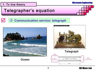
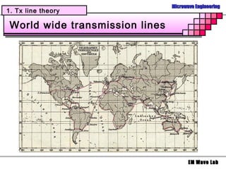
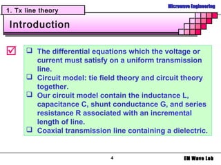
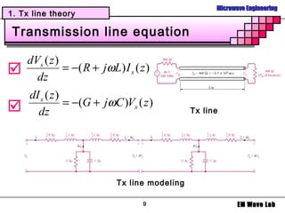
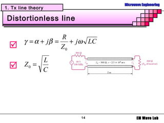
1. Tx line theory
Circuit model
ˆ
Propagation in the a z direction
Length ∆z : R∆z[ Ω], L∆z[ H ], G∆z[1 / Ω], C∆z[ F ]
lim: infinitesimal approach
∆z →0
7 EM Wave Lab](https://image.slidesharecdn.com/5-transmissionline-120810003450-phpapp01/85/Transmission-Line-7-320.jpg)


![Microwave Engineering
2. Tx line parameters
Coaxial line
ρL
∫S D • dS = Q 2πρLD = ρ L L D = 2πρ a ρ
ρL
E= aρ
2πε ' ρ
a ρL ρ ρ b
Vo = − ∫
a
dρ = − L ln ρ b = L ln
b 2πε ' ρ 2πε ' 2πε ' a
Cross section
2πε
C= [ F/m]
ln(b / a )
Coaxial line + connector
28 EM Wave Lab](https://image.slidesharecdn.com/5-transmissionline-120810003450-phpapp01/85/Transmission-Line-28-320.jpg)
![Microwave Engineering
2. Tx line parameters
Coaxial line
ε C ε σ 2πσ
RC = , = , G = C ⇒ G = [1 / Ωm]
σ G σ ε ln(b / a)
µId b µ b
Φ= ln , Lext = ln [ H / m]
2π a 2π a
1 1 1 1 1
Rinner = , Router = ⇒R= + [ Ω / m]
2πaδσ c 2πbδσ c 2πδσ c a b
The characteristic impedance of a coax
Lext 1 µ b
Z0 = = ln
C 2π ε a
29 EM Wave Lab](https://image.slidesharecdn.com/5-transmissionline-120810003450-phpapp01/85/Transmission-Line-29-320.jpg)

1. The document discusses transmission line theory and parameters. Key topics covered include: - Telegrapher's equation and circuit model for transmission lines - Wave propagation and characteristic impedance calculations - Reflection coefficient and standing wave ratio definitions - Comparisons of transmission line, circuit, and field theories 2. Specific transmission line types are analyzed, including planar lines, coaxial cables. Equations are given for calculating the capacitance, conductance, inductance, resistance, and characteristic impedance of these common line configurations. 3. Simulation and modeling techniques for transmission lines are briefly mentioned, such as the transmission line matrix method for modeling microstrip lines in antennas and circuits.


![RF Circuit Design - [Ch1-2] Transmission Line Theory](https://cdn.slidesharecdn.com/ss_thumbnails/ch1-2-150613064349-lva1-app6892-thumbnail.jpg?width=640&height=640&fit=bounds)
![RF Circuit Design - [Ch3-1] Microwave Network](https://cdn.slidesharecdn.com/ss_thumbnails/ch3-1-150613064402-lva1-app6892-thumbnail.jpg?width=640&height=640&fit=bounds)
![RF Circuit Design - [Ch2-2] Smith Chart](https://cdn.slidesharecdn.com/ss_thumbnails/ch2-2-150613064401-lva1-app6891-thumbnail.jpg?width=640&height=640&fit=bounds)
![RF Circuit Design - [Ch2-1] Resonator and Impedance Matching](https://cdn.slidesharecdn.com/ss_thumbnails/ch2-1-150613064353-lva1-app6892-thumbnail.jpg?width=640&height=640&fit=bounds)
![RF Circuit Design - [Ch4-2] LNA, PA, and Broadband Amplifier](https://cdn.slidesharecdn.com/ss_thumbnails/ch4-2-150613064410-lva1-app6891-thumbnail.jpg?width=640&height=640&fit=bounds)
![RF Circuit Design - [Ch4-1] Microwave Transistor Amplifier](https://cdn.slidesharecdn.com/ss_thumbnails/ch4-1-150613064409-lva1-app6892-thumbnail.jpg?width=640&height=640&fit=bounds)


![RF Circuit Design - [Ch1-1] Sinusoidal Steady-state Analysis](https://cdn.slidesharecdn.com/ss_thumbnails/ch1-1-150613064348-lva1-app6891-thumbnail.jpg?width=640&height=640&fit=bounds)

![RF Module Design - [Chapter 2] Noises](https://cdn.slidesharecdn.com/ss_thumbnails/rfch2-150613070344-lva1-app6892-thumbnail.jpg?width=640&height=640&fit=bounds)
![RF Module Design - [Chapter 3] Linearity](https://cdn.slidesharecdn.com/ss_thumbnails/rfch3-150613070345-lva1-app6891-thumbnail.jpg?width=640&height=640&fit=bounds)


![RF Module Design - [Chapter 5] Low Noise Amplifier](https://cdn.slidesharecdn.com/ss_thumbnails/rfch5-150613070346-lva1-app6891-thumbnail.jpg?width=640&height=640&fit=bounds)
![RF Module Design - [Chapter 4] Transceiver Architecture](https://cdn.slidesharecdn.com/ss_thumbnails/rfch4-150613070346-lva1-app6891-thumbnail.jpg?width=640&height=640&fit=bounds)


![射頻電子 - [第二章] 傳輸線理論](https://cdn.slidesharecdn.com/ss_thumbnails/ch2-150613065059-lva1-app6891-thumbnail.jpg?width=640&height=640&fit=bounds)


