This document summarizes key concepts in propagation models for wireless mobile communications. It discusses free space losses, plane earth losses, and models for the wireless channel including macrocells, shadowing, narrowband fast fading, and wideband fast fading. Empirical and physical statistical models are described for modeling propagation in different environments like urban, suburban, and rural areas. Deterministic and statistical models are presented for modeling narrowband fast fading effects.
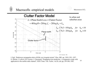
![Microwaves UCL
37
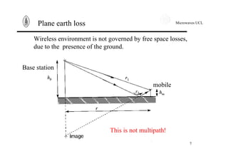
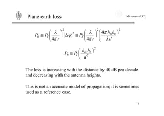
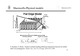
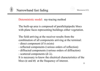
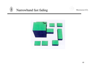
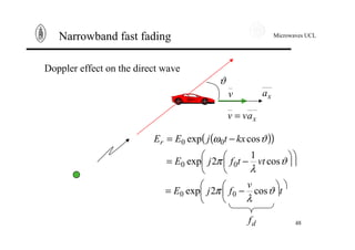
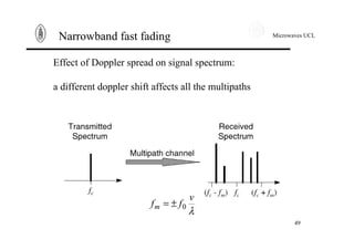
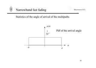
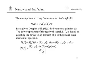
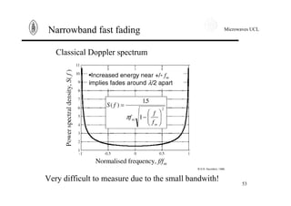
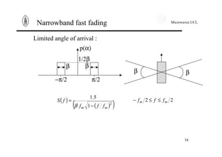
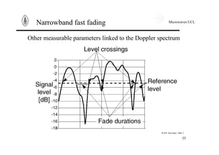
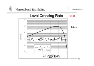
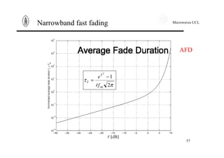
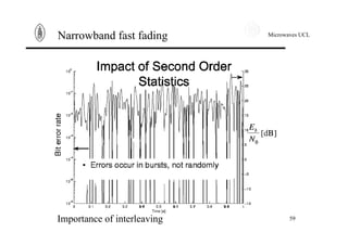
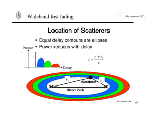
Narrowband fast fading
30 40 50 60 70 80 90
−60
−55
−50
−45
−40
−35
−30
12.5 GHz
Distance from Maxwell building, [m]
Receivedpower,[dB]
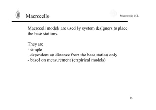
30 40 50 60 70 80 90
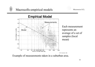
−65
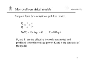
−60
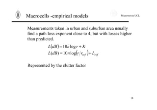
−55
−50
−45
−40
−35
−30
30 GHz
Distance from Maxwell building, [m]
Receivedpower,[dB]
+
Simulation winter
Simulation summer
Meas. winter
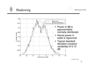
Meas. summer
Comparison between simulation and measurement](https://image.slidesharecdn.com/propagationmodel-12704657499131-phpapp01/85/Propagation-Model-37-320.jpg)
![Microwaves UCL
60
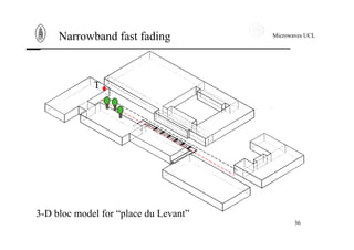
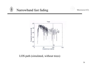
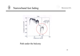
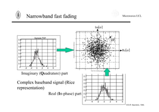
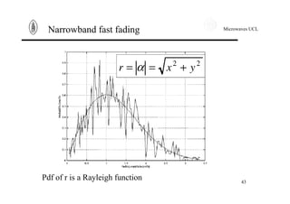
Narrowband fast fading
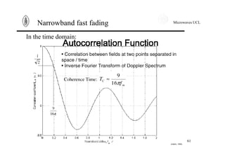
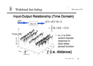
Another way to see Doppler effect is to work in time domain.
The inverse Fourier Transform of the power spectral density is
the autocorrelation function. It expresses correlation between a
signal at t and its value at t+τ. The autocorrelation function of
the received signal writes down
( ) ( ) ( )[ ] [ ]2*
αταατρ EttE +=
For the classical spectrum, one obtains
( ) ( )τπρ mfJt 20=
The coherence time is defined as the time during which teh
channel can be considered as constant. The signals, shorter then
the coherence time are not affected by the Doppler shift nor the
speed of the mobile.](https://image.slidesharecdn.com/propagationmodel-12704657499131-phpapp01/85/Propagation-Model-60-320.jpg)
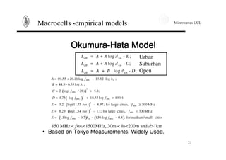
![Microwaves UCL
81
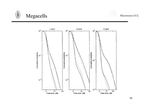
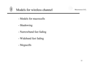
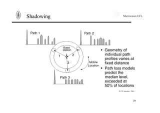
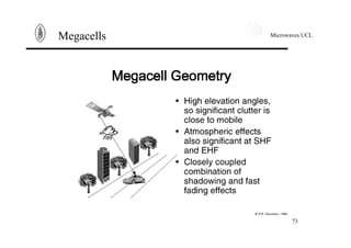
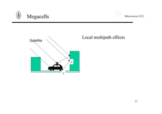
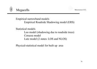
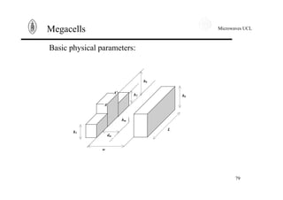
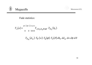
Megacells
0 2 4 6 8 10 12 14 16 18 20
0
0.05
0.1
0.15
0.2
0.25
0.3
Building height, [m]
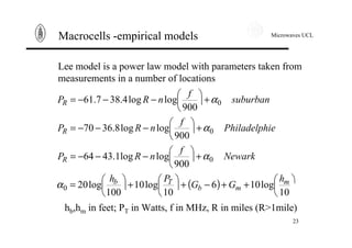
Probabilitydensityfunction
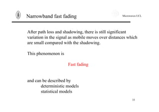
Guildford
Building height distribution](https://image.slidesharecdn.com/propagationmodel-12704657499131-phpapp01/85/Propagation-Model-81-320.jpg)
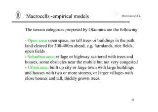
![Microwaves UCL
82
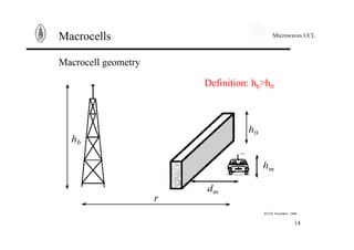
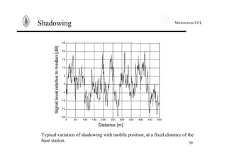
Megacells
5 15 25 35 45 55 65 75 85
0
0.005
0.01
0.015
0.02
0.025
0.03
0.035
0.04
Elevation angle, [deg.]
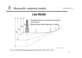
Probabilitydensityfunction
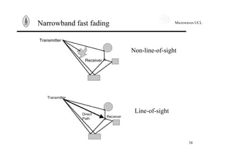
Maximum elevation angle
for Iridium constellation
at London](https://image.slidesharecdn.com/propagationmodel-12704657499131-phpapp01/85/Propagation-Model-82-320.jpg)
![Microwaves UCL
83
Megacells
0 10 20 30 40 50 60
0
0.01
0.02
0.03
0.04
0.05
0.06
0.07
Street width, [m]
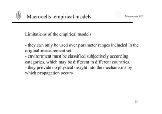
Probabilitydensityfunction
Street width distribution in
Guildford](https://image.slidesharecdn.com/propagationmodel-12704657499131-phpapp01/85/Propagation-Model-83-320.jpg)
![Microwaves UCL
84
Megacells
0 1 2 3 4 5 6
0
0.05
0.1
0.15
0.2
0.25
0.3
0.35
Satellite azimuth angle, [rad.]
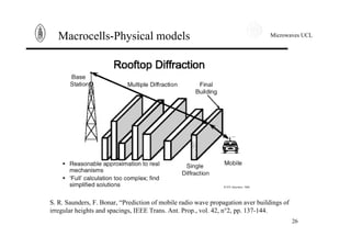
Probabilitydensity
Distribution of the nearest satellite azimuth
angle (relative to earth parallels) for Iridium at
London](https://image.slidesharecdn.com/propagationmodel-12704657499131-phpapp01/85/Propagation-Model-84-320.jpg)
![Microwaves UCL
85
Megacells
0 1 2 3 4 5 6
0.15
0.152
0.154
0.156
0.158
0.16
0.162
0.164
0.166
0.168
0.17
Satellite azimuth angle, [rad.]
Probabilitydensity Distribution of the global azimuth angle (relative to
street axis) for Iridium constellation at London](https://image.slidesharecdn.com/propagationmodel-12704657499131-phpapp01/85/Propagation-Model-85-320.jpg)