Downloaded 255 times

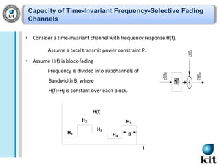
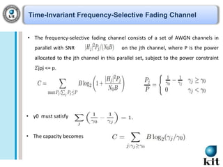
![Shannon Capacity and Mutual Information
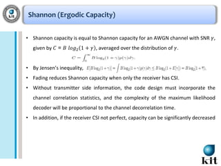
• Shannon defined capacity as the maximum mutual information of channel.
• Maximum error-free data rate a channel can support.
• Mutual information :
• Mutual information measures the information that X and Y share: it
measures how many knowing on of these variables reduces uncertainty
about the other [1].](https://image.slidesharecdn.com/chapter4-131118201118-phpapp02/85/Wireless-Channels-Capacity-2-320.jpg)
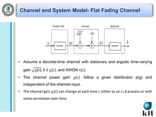
![Channel and System Model (Cont…)
• In block fading channel g[i] is constant over some blocklength T after
which time g[i] changes to a new independent value based on the
distribution p(g).
• Let P denote the average transmit signal power, 𝑁0 /2 denote the noise
spectral density of n[i], and B denote the received signal bandwidth.
• The instantaneous received signal-to-noise ratio (SNR) is,
and its expected value over all time is
.](https://image.slidesharecdn.com/chapter4-131118201118-phpapp02/85/Wireless-Channels-Capacity-5-320.jpg)
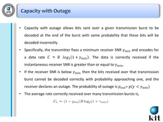
![Capacity of Flat-Fading Channels
We will consider 3 different scenarios :
1. Channel Distribution Information (CDI) : The distribution of g[i] is known to
the transmitter and receiver.
2. Receiver CSI : The value of g[i] is known at the receiver at time i, and both
the transmitter and receiver know the distribution of g[i].
3. Transmitter and Receiver CSI : The value of g[i] is known at the transmitter
and receiver at time i, and both the transmitter and receiver know the
distribution of g[i].](https://image.slidesharecdn.com/chapter4-131118201118-phpapp02/85/Wireless-Channels-Capacity-6-320.jpg)
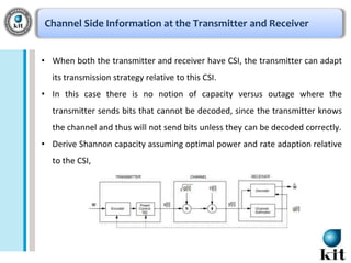
![Channel Side Information at Receiver
• The value of g[i] is known at the receiver at time i, and both the transmitter
and receiver know the distribution of g[i].
• In this case there are two channel capacity that are relevant to system design:
Shannon (ergodic) capacity and capacity with outage.
• Shannon capacity the rate transmitter over the channel is constant.
• Capacity with outage is defined as the maximum rate that can be transmitted
over a channel with some outage probability corresponding to the probability
that the transmission cannot be decoded with negligible error probability.](https://image.slidesharecdn.com/chapter4-131118201118-phpapp02/85/Wireless-Channels-Capacity-7-320.jpg)
![Shannon Capacity
• Consider the Shannon capacity when the channel power gain g[i] is known to
both the transmitter and receiver at time i.
• Let us now allow the transmit power S(𝛾) to vary with 𝛾, subject to an
average power constraint 𝑆:](https://image.slidesharecdn.com/chapter4-131118201118-phpapp02/85/Wireless-Channels-Capacity-11-320.jpg)

![Zero-Outage Capacity and Channel Inversion
Zero-Outage Capacity
• Fading inverted to maintain constant SNR.
• Simplifies design (fixed rate).
• Since the data rate is fixed under all channel conditions and there is no channel
outage.
Channel Inversion
• Suboptimal transmitter adaptation scheme where the transmitter uses the CSI to
maintain a constant received power.
• This power adaptation, called channel inversion, is given by P(γ)/P = 𝜎/γ, where 𝜎
equals the constant received SNR that can be maintained with the transmit power
constraint. 𝜎 satisfies 𝜎 =1/E[1/γ].
• In Rayleigh fading E[1/γ] is infinite, and thus the zero-outage capacity given by is zero.](https://image.slidesharecdn.com/chapter4-131118201118-phpapp02/85/Wireless-Channels-Capacity-16-320.jpg)
![Outage Capacity and Truncated Channel Inversion
• The outage capacity is defined as the maximum data rate that can be maintained
by suspending transmission in bad fading states.
• We can maintain a higher constant data rate in the other state and can increase
the channel capacity.
• Outage Capacity is achieved with a truncated inversion policy for power
adaption which only compensates for fading above a certain cutoff fade depth
γ0:
• where γ0 is based on the outage probability: pout= p(γ<γ0). Since the channel is
only used when γ >= γ0, 𝜎 =1/Eγ0 [1/γ], where](https://image.slidesharecdn.com/chapter4-131118201118-phpapp02/85/Wireless-Channels-Capacity-17-320.jpg)
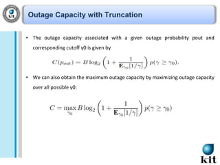
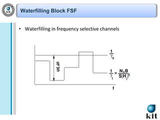
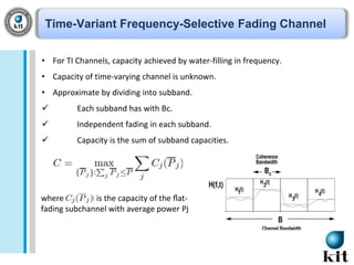

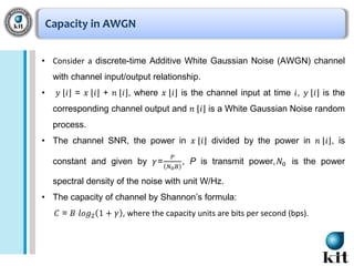
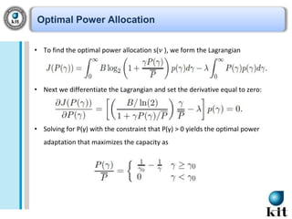
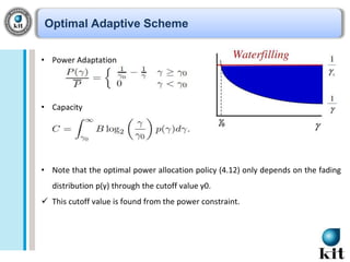
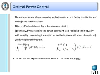
1) The document discusses the capacity of wireless channels, including Shannon capacity, capacity in additive white Gaussian noise (AWGN) channels, and capacity of flat fading channels with different channel state information scenarios. 2) It describes the optimal power allocation strategy when the transmitter and receiver have channel state information, which is to allocate more power to better channel states using waterfilling. 3) For frequency-selective fading channels, capacity is achieved through waterfilling in frequency to allocate higher power to better subchannels subject to an overall power constraint.