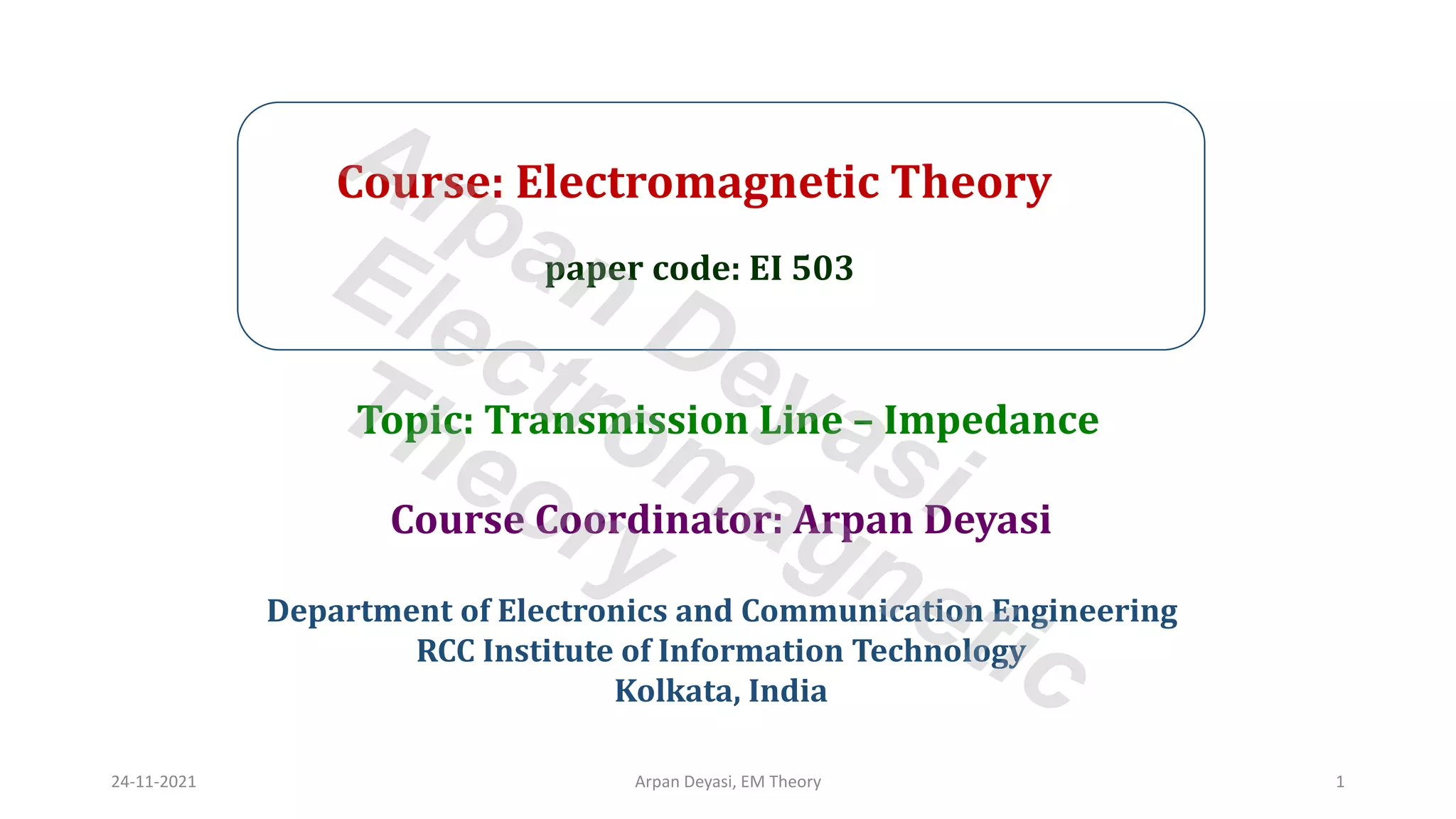
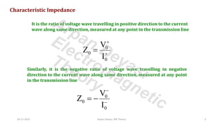
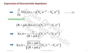
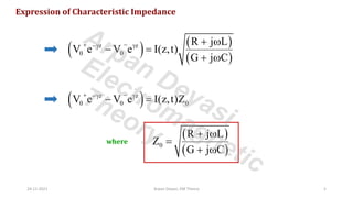
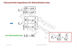
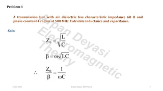
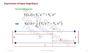
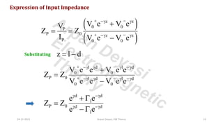
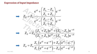
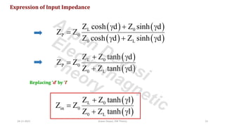
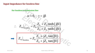
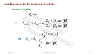
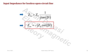
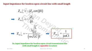
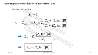
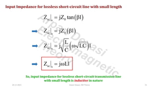
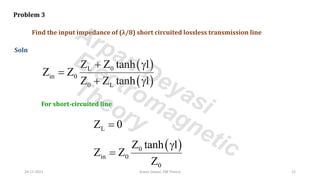
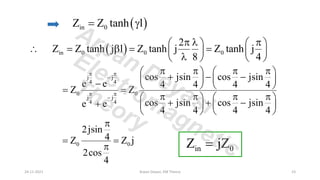
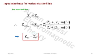
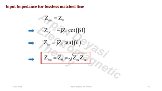
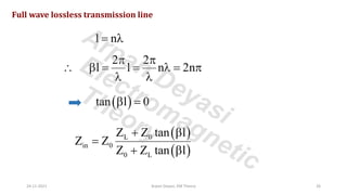
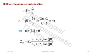
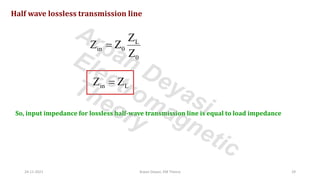
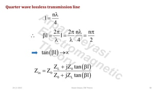
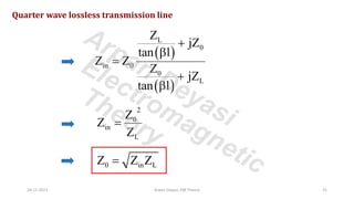
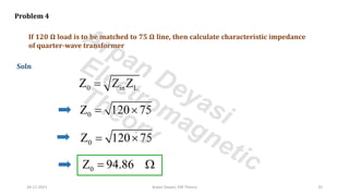
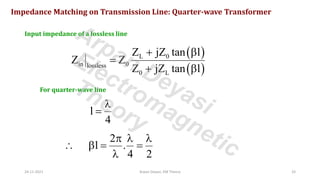
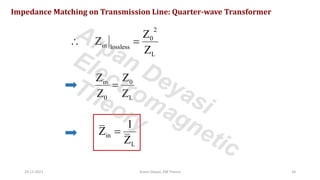
Course: Electromagnetic Theory
paper code: EI 503
Course Coordinator: Arpan Deyasi
Department of Electronics and Communication Engineering
RCC Institute of Information Technology
Kolkata, India
Topic: Transmission Line – Impedance
24-11-2021 Arpan Deyasi, EM Theory 1
Arpan Deyasi
Electromagnetic
Theory
Characteristic Impedance
It is the ratio of voltage wave travelling in positive direction to the current
wave along same direction, measured at any point in the transmission line
0
0
0
V
Z
I
+
+
=
Similarly, it is the negative ratio of voltage wave travelling in negative
direction to the current wave along same direction, measured at any point
in the transmission line
0
0
0
V
Z
I
−
−
= −
24-11-2021 Arpan Deyasi, EM Theory 2
Arpan Deyasi
Electromagnetic
Theory
Expression of Characteristic Impedance
From transmission line equation
V(z,t) RI(z,t) L I(z,t)
z t
 
− = +
 
Substituting j
t

 

( )
V(z,t) R j L I(z,t)
z

− = + 

Now z z
0 0
V(z,t) V e V e
+ −
− 
= +
…………….. (1)
24-11-2021 Arpan Deyasi, EM Theory 3
Arpan Deyasi
Electromagnetic
Theory
Expression of Characteristic Impedance
( )
z z
0 0
V(z,t) V e V e
z
+ −
− 

= − −

…………….. (2)
Substituting in (1)
( ) ( )
z z
0 0
R j L I(z,t) V e V e
+ −
− 
+  =  −
( )
( )
z z
0 0
I(z,t) V e V e
R j L
+ −
− 

= −
+ 
( )
( )
( )
z z
0 0
G j C
I(z,t) V e V e
R j L
+ −
− 
+ 
= −
+ 
24-11-2021 Arpan Deyasi, EM Theory 4
Arpan Deyasi
Electromagnetic
Theory
Expression of Characteristic Impedance
( ) ( )
( )
z z
0 0
R j L
V e V e I(z,t)
G j C
+ −
−  + 
− =
+ 
( )
z z
0 0 0
V e V e I(z,t)Z
+ −
− 
− =
where
( )
( )
0
R j L
Z
G j C
+ 
=
+ 
24-11-2021 Arpan Deyasi, EM Theory 5
Arpan Deyasi
Electromagnetic
Theory
Characteristic Impedance for Distortionless Line
( )
( )
0
R j L
Z
G j C
+ 
=
+ 
0
L
R 1 j
R
Z
C
G 1 j
G
 
+ 
 
 
=
 
+ 
 
 
LG RC
=
For distortionless line
0
R L
Z
G C
 = =
24-11-2021 Arpan Deyasi, EM Theory 6
Arpan Deyasi
Electromagnetic
Theory
A transmission line with air dielectric has characteristic impedance 60 Ω and
phase constant 4 rad/m at 500 MHz. Calculate inductance and capacitance.
Problem 1
Soln
0
L
Z
C
=
LC
 = 
0
Z 1
C
 =
 
24-11-2021 Arpan Deyasi, EM Theory 7
Arpan Deyasi
Electromagnetic
Theory
0
C 21.2 pF/m
Z

= =

2
0
L Z C 334.2 mH/m
= =
24-11-2021 Arpan Deyasi, EM Theory 8
Arpan Deyasi
Electromagnetic
Theory
A distortionless line has Z0 = 60 Ω, α = 20 mNp/m, u = 0.6c. Find R, L, G, C at 100
MHz.
Problem 2
Soln
0
L
Z 60
C
= =
3
C
R 20 10
L
−
 = = 
R 1.2 /m
 = 
24-11-2021 Arpan Deyasi, EM Theory 9
Arpan Deyasi
Electromagnetic
Theory
8
p
1
v 0.6 3 10
LC
= =  
0
L
Z 60
C
= =
L 333.3 nH/m
 =
& C 92.59 pF/m
=
24-11-2021 Arpan Deyasi, EM Theory 10
Arpan Deyasi
Electromagnetic
Theory
0
R
Z 60
G
= =
R 1.2 /m
= 
G 333.3 S/m
 = 
24-11-2021 Arpan Deyasi, EM Theory 11
Arpan Deyasi
Electromagnetic
Theory
Expression of Input Impedance
For travelling wave
z z
0 0
V(z,t) V e V e
+ −
− 
= +
( )
z z
0 0
0
1
I(z,t) V e V e
Z
+ −
− 
= −
S L
P
z
d
l
24-11-2021 Arpan Deyasi, EM Theory 12
Arpan Deyasi
Electromagnetic
Theory
Expression of Input Impedance
( )
( )
z z
0 0
P
P 0 z z
P 0 0
V e V e
V
Z Z
I V e V e
+ −
− 
+ −
− 
+
= =
−
Substituting z l d
= −
l d l d
0 0
P 0 l d l d
0 0
V e e V e e
Z Z
V e e V e e
+ −
−   −
+ −
−   −
+
=
−
d d
l
P 0 d d
l
e e
Z Z
e e
 −
 −
+ 
=
− 
24-11-2021 Arpan Deyasi, EM Theory 13
Arpan Deyasi
Electromagnetic
Theory
d d
L 0
L 0
P 0
d d
L 0
L 0
Z Z
e e
Z Z
Z Z
Z Z
e e
Z Z
 −
 −
 
−
+  
+
 
=
 
−
−  
+
 
Expression of Input Impedance
( ) ( )
( ) ( )
d d
L 0 L 0
P 0 d d
L 0 L 0
Z Z e Z Z e
Z Z
Z Z e Z Z e
 −
 −
+ + −
=
+ − −
( ) ( )
( ) ( )
d d d d
L 0
P 0 d d d d
L 0
Z e e Z e e
Z Z
Z e e Z e e
 −  −
 −  −
+ + −
=
+ − −
24-11-2021 Arpan Deyasi, EM Theory 14
Arpan Deyasi
Electromagnetic
Theory
Expression of Input Impedance
( ) ( )
( ) ( )
L 0
P 0
0 L
Z cosh d Z sinh d
Z Z
Z cosh d Z sinh d
 + 
=
 + 
( )
( )
L 0
P 0
0 L
Z Z tanh d
Z Z
Z Z tanh d
+ 
=
+ 
Replacing ‘d’ by ‘l’
( )
( )
L 0
in 0
0 L
Z Z tanh l
Z Z
Z Z tanh l
+ 
=
+ 
24-11-2021 Arpan Deyasi, EM Theory 15
Arpan Deyasi
Electromagnetic
Theory
Input Impedance for lossless line
For lossless transmission line
0, j
 =  = 
( )
( )
L 0
in 0
lossless
0 L
Z Z tanh j l
Z Z
Z Z tanh j l
+ 
 =
+ 
( )
( )
L 0
in 0
lossless
0 L
Z jZ tan l
Z Z
Z jZ tan l
+ 
=
+ 
24-11-2021 Arpan Deyasi, EM Theory 16
Arpan Deyasi
Electromagnetic
Theory
Input Impedance for lossless open-circuit line
For open-circuit line
L
Z →
( )
( )
L 0
inll oc 0
o.c
0 L
Z jZ tan l
Z Z Z
Z jZ tan l
+ 
 = =
+ 
( )
( )
0
L
oc 0
0
L
Z
1 j tan l
Z
Z Z
Z
jtan l
Z
+ 
=
+ 
24-11-2021 Arpan Deyasi, EM Theory 17
Arpan Deyasi
Electromagnetic
Theory
Input Impedance for lossless open-circuit line
( )
oc 0
1
Z Z
jtan l
=

( )
oc 0
Z jZ cot l
= − 
24-11-2021 Arpan Deyasi, EM Theory 18
Arpan Deyasi
Electromagnetic
Theory
Input Impedance for lossless open-circuit line with small length
( )
oc 0
s
Z jZ cot l
= − 
0
oc s
jZ
Z
l
= −

( )
oc s
L
j
C
Z
LC l
= −

oc s
1
Z
j Cl
=

So, input impedance for lossless open-circuit transmission line
with small length is capacitive in nature
24-11-2021 Arpan Deyasi, EM Theory 19
Arpan Deyasi
Electromagnetic
Theory
Input Impedance for lossless short-circuit line
For short-circuit line
L
Z 0
=
( )
( )
L 0
inll sc 0
s.c
0 L
Z jZ tan l
Z Z Z
Z jZ tan l
+ 
 = =
+ 
( )
0
sc 0
0
jZ tan l
Z Z
Z

=
( )
sc 0
Z jZ tan l
= 
24-11-2021 Arpan Deyasi, EM Theory 20
Arpan Deyasi
Electromagnetic
Theory
Input Impedance for lossless short-circuit line with small length
( )
sc 0
s
Z jZ tan l
= 
( )
sc 0
s
Z jZ l
= 
( )
sc s
L
Z j LC l
C
= 
sc s
Z j Ll
= 
So, input impedance for lossless short-circuit transmission line
with small length is inductive in nature
24-11-2021 Arpan Deyasi, EM Theory 21
Arpan Deyasi
Electromagnetic
Theory
Problem 3
Find the input impedance of (λ/8) short circuited lossless transmission line
Soln
( )
( )
L 0
in 0
0 L
Z Z tanh l
Z Z
Z Z tanh l
+ 
=
+ 
For short-circuited line
L
Z 0
=
( )
0
in 0
0
Z tanh l
Z Z
Z

=
24-11-2021 Arpan Deyasi, EM Theory 22
Arpan Deyasi
Electromagnetic
Theory
( )
in 0
Z Z tanh l
= 
( )
in 0 0 0
2
Z Z tanh j l Z tanh j Z tanh j
8 4
  
   
 =  = =
   

   
j j
4 4
0 0
j j
4 4
cos jsin cos jsin
e e 4 4 4 4
Z Z
cos jsin cos jsin
e e
4 4 4 4
 
−
 
−
   
   
+ − −
   
−    
= =
   
   
+ + −
+    
   
0 0
2jsin
4
Z Z j
2cos
4

= =
 in 0
Z jZ
=
24-11-2021 Arpan Deyasi, EM Theory 23
Arpan Deyasi
Electromagnetic
Theory
Input Impedance for lossless matched line
For matched line
L 0
Z Z
=
( )
( )
L 0
inll mc 0
m.c
0 L
Z jZ tan l
Z Z Z
Z jZ tan l
+ 
 = =
+ 
mc 0
Z Z
=
24-11-2021 Arpan Deyasi, EM Theory 24
Arpan Deyasi
Electromagnetic
Theory
Input Impedance for lossless matched line
mc 0
Z Z
=
( )
oc 0
Z jZ cot l
= − 
( )
sc 0
Z jZ tan l
= 
mc 0 oc sc
Z Z Z Z
= =
24-11-2021 Arpan Deyasi, EM Theory 25
Arpan Deyasi
Electromagnetic
Theory
Full wave lossless transmission line
l n
= 
2 2
l l n 2n
 
  = =  = 
 
( )
tan l 0
 =
( )
( )
L 0
in 0
0 L
Z Z tan l
Z Z
Z Z tan l
+ 
=
+ 
24-11-2021 Arpan Deyasi, EM Theory 26
Arpan Deyasi
Electromagnetic
Theory
Full wave lossless transmission line
L
in 0
0
Z
Z Z
Z
=
in L
Z Z
=
So, input impedance for lossless full-wave transmission line is equal to load impedance
24-11-2021 Arpan Deyasi, EM Theory 27
Arpan Deyasi
Electromagnetic
Theory
n
l
2

=
2 2 n
l l n
2
  
  = = = 
 
( )
tan l 0
 =
( )
( )
L 0
in 0
0 L
Z jZ tan l
Z Z
Z jZ tan l
+ 
=
+ 
Half wave lossless transmission line
24-11-2021 Arpan Deyasi, EM Theory 28
Arpan Deyasi
Electromagnetic
Theory
Half wave lossless transmission line
L
in 0
0
Z
Z Z
Z
=
in L
Z Z
=
So, input impedance for lossless half-wave transmission line is equal to load impedance
24-11-2021 Arpan Deyasi, EM Theory 29
Arpan Deyasi
Electromagnetic
Theory
Quarter wave lossless transmission line
n
l
4

=
2 2 n n
l l
4 2
   
  = = =
 
( )
tan l
 →
( )
( )
L 0
in 0
0 L
Z jZ tan l
Z Z
Z jZ tan l
+ 
=
+ 
24-11-2021 Arpan Deyasi, EM Theory 30
Arpan Deyasi
Electromagnetic
Theory
Quarter wave lossless transmission line
( )
( )
L
0
in 0
0
L
Z
jZ
tan l
Z Z
Z
jZ
tan l
+

=
+

2
0
in
L
Z
Z
Z
=
0 in L
Z Z Z
=
24-11-2021 Arpan Deyasi, EM Theory 31
Arpan Deyasi
Electromagnetic
Theory
If 120 Ω load is to be matched to 75 Ω line, then calculate characteristic impedance
of quarter-wave transformer
Problem 4
Soln
0 in L
Z Z Z
=
0
Z 120 75
= 
0
Z 120 75
= 
0
Z 94.86
= 
24-11-2021 Arpan Deyasi, EM Theory 32
Arpan Deyasi
Electromagnetic
Theory
24-11-2021 Arpan Deyasi, EM Theory 33
Impedance Matching on Transmission Line: Quarter-wave Transformer
Input impedance of a lossless line
( )
( )
L 0
in 0
lossless
0 L
Z jZ tan l
Z Z
Z jZ tan l
+ 
=
+ 
For quarter-wave line
l
4

=
2
l .
4 2
  
  = =

Arpan Deyasi
Electromagnetic
Theory
24-11-2021 Arpan Deyasi, EM Theory 34
2
0
in lossless
L
Z
Z
Z
 =
in 0
0 L
Z Z
Z Z
=
in
L
1
Z
Z
=
Impedance Matching on Transmission Line: Quarter-wave Transformer
Arpan Deyasi
Electromagnetic
Theory
24-11-2021 Arpan Deyasi, EM Theory 35
Impedance Matching on Transmission Line: Quarter-wave Transformer
1. Normalized input impedance of a λ/4 transmission line is equal to the reciprocal of
normalized terminating impedance. Therefore, a quarter-wave section can be considered
as impedance converter between high to low and vice-versa.
2. Short-circuited λ/4 transmission line has infinite input impedance.
3. Open-circuited λ/4 transmission line has zero input impedance.
Drawback of this technique is that it needs special line of characteristics
impedance for every pair of resistances to be matched.
Arpan Deyasi
Electromagnetic
Theory
24-11-2021 Arpan Deyasi, EM Theory 36
Stub
A stub is a short-circuited section of a transmission line connected in parallel to the
main transmission line.
A stub of appropriate length is placed at some distance from the load such that the
impedance seen beyond the stub is equal to the characteristic impedance.
Use of stub
Stubs can be used to match a load impedance to the transmission line characteristic
impedance
Arpan Deyasi
Electromagnetic
Theory
24-11-2021 Arpan Deyasi, EM Theory 37
Impedance Matching on Transmission Line: Single stub matching
The single-stub matching technique is superior to the quarter wavelength
transformer as it makes use of only one type of transmission line for the main
line as well as the stub.
This technique also in principle is capable of matching any complex load to the
characteristic impedance/admittance.
The single stub matching technique is quite popular in matching fixed
impedances at microwave frequencies.
Arpan Deyasi
Electromagnetic
Theory
24-11-2021 Arpan Deyasi, EM Theory 38
Impedance Matching on Transmission Line: Single stub matching
ZL
Z0
l1
l2
Arpan Deyasi
Electromagnetic
Theory
24-11-2021 Arpan Deyasi, EM Theory 39
Impedance Matching on Transmission Line: Single stub matching
Suppose we have a load impedance ZL connected to a transmission line with
characteristic impedance Z0
The objective here is that no reflection should be seen by the generator. In other
words, even if there are standing waves in the vicinity of the load , the standing
waves must vanish beyond certain distance from the load.
Conceptually this can be achieved by adding a stub to the main line such that the
reflected wave from the short-circuit end of the stub and the reflected wave from
the load on the main line completely cancel each other.
Arpan Deyasi
Electromagnetic
Theory
24-11-2021 Arpan Deyasi, EM Theory 40
Impedance Matching on Transmission Line: Single stub matching
The single stub matching technique although has overcome the drawback of the
quarter wavelength transformer technique, it still is not suitable for matching
variable impedances.
A change in load impedance results in a change in the length as well as the location
of the stub.
Even if changing length of a stub is a simpler task, changing the location of a stub
may not be easy in certain transmission line configurations.
Drawbacks Arpan Deyasi
Electromagnetic
Theory
24-11-2021 Arpan Deyasi, EM Theory 41
Impedance Matching on Transmission Line: Double stub matching
ZL
Z0
l1
l3
l2
Arpan Deyasi
Electromagnetic
Theory
24-11-2021 Arpan Deyasi, EM Theory 42
Impedance Matching on Transmission Line: Double stub matching
The technique uses two stubs with fixed locations.
As the load changes only the lengths of the stubs are adjusted to achieve matching.
Let us assume that a normalized admittance is to be matched using the double stub
matching technique. The first stub is located at a convenient distance from the load.
The second stub is located at a distance of 3λ/8 rom the first stub.
Arpan Deyasi
Electromagnetic
Theory

Impedance in transmission line

  • 1.
    Course: Electromagnetic Theory papercode: EI 503 Course Coordinator: Arpan Deyasi Department of Electronics and Communication Engineering RCC Institute of Information Technology Kolkata, India Topic: Transmission Line – Impedance 24-11-2021 Arpan Deyasi, EM Theory 1 Arpan Deyasi Electromagnetic Theory
  • 2.
    Characteristic Impedance It isthe ratio of voltage wave travelling in positive direction to the current wave along same direction, measured at any point in the transmission line 0 0 0 V Z I + + = Similarly, it is the negative ratio of voltage wave travelling in negative direction to the current wave along same direction, measured at any point in the transmission line 0 0 0 V Z I − − = − 24-11-2021 Arpan Deyasi, EM Theory 2 Arpan Deyasi Electromagnetic Theory
  • 3.
    Expression of CharacteristicImpedance From transmission line equation V(z,t) RI(z,t) L I(z,t) z t   − = +   Substituting j t     ( ) V(z,t) R j L I(z,t) z  − = +   Now z z 0 0 V(z,t) V e V e + − −  = + …………….. (1) 24-11-2021 Arpan Deyasi, EM Theory 3 Arpan Deyasi Electromagnetic Theory
  • 4.
    Expression of CharacteristicImpedance ( ) z z 0 0 V(z,t) V e V e z + − −   = − −  …………….. (2) Substituting in (1) ( ) ( ) z z 0 0 R j L I(z,t) V e V e + − −  +  =  − ( ) ( ) z z 0 0 I(z,t) V e V e R j L + − −   = − +  ( ) ( ) ( ) z z 0 0 G j C I(z,t) V e V e R j L + − −  +  = − +  24-11-2021 Arpan Deyasi, EM Theory 4 Arpan Deyasi Electromagnetic Theory
  • 5.
    Expression of CharacteristicImpedance ( ) ( ) ( ) z z 0 0 R j L V e V e I(z,t) G j C + − −  +  − = +  ( ) z z 0 0 0 V e V e I(z,t)Z + − −  − = where ( ) ( ) 0 R j L Z G j C +  = +  24-11-2021 Arpan Deyasi, EM Theory 5 Arpan Deyasi Electromagnetic Theory
  • 6.
    Characteristic Impedance forDistortionless Line ( ) ( ) 0 R j L Z G j C +  = +  0 L R 1 j R Z C G 1 j G   +      =   +      LG RC = For distortionless line 0 R L Z G C  = = 24-11-2021 Arpan Deyasi, EM Theory 6 Arpan Deyasi Electromagnetic Theory
  • 7.
    A transmission linewith air dielectric has characteristic impedance 60 Ω and phase constant 4 rad/m at 500 MHz. Calculate inductance and capacitance. Problem 1 Soln 0 L Z C = LC  =  0 Z 1 C  =   24-11-2021 Arpan Deyasi, EM Theory 7 Arpan Deyasi Electromagnetic Theory
  • 8.
    0 C 21.2 pF/m Z  ==  2 0 L Z C 334.2 mH/m = = 24-11-2021 Arpan Deyasi, EM Theory 8 Arpan Deyasi Electromagnetic Theory
  • 9.
    A distortionless linehas Z0 = 60 Ω, α = 20 mNp/m, u = 0.6c. Find R, L, G, C at 100 MHz. Problem 2 Soln 0 L Z 60 C = = 3 C R 20 10 L −  = =  R 1.2 /m  =  24-11-2021 Arpan Deyasi, EM Theory 9 Arpan Deyasi Electromagnetic Theory
  • 10.
    8 p 1 v 0.6 310 LC = =   0 L Z 60 C = = L 333.3 nH/m  = & C 92.59 pF/m = 24-11-2021 Arpan Deyasi, EM Theory 10 Arpan Deyasi Electromagnetic Theory
  • 11.
    0 R Z 60 G = = R1.2 /m =  G 333.3 S/m  =  24-11-2021 Arpan Deyasi, EM Theory 11 Arpan Deyasi Electromagnetic Theory
  • 12.
    Expression of InputImpedance For travelling wave z z 0 0 V(z,t) V e V e + − −  = + ( ) z z 0 0 0 1 I(z,t) V e V e Z + − −  = − S L P z d l 24-11-2021 Arpan Deyasi, EM Theory 12 Arpan Deyasi Electromagnetic Theory
  • 13.
    Expression of InputImpedance ( ) ( ) z z 0 0 P P 0 z z P 0 0 V e V e V Z Z I V e V e + − −  + − −  + = = − Substituting z l d = − l d l d 0 0 P 0 l d l d 0 0 V e e V e e Z Z V e e V e e + − −   − + − −   − + = − d d l P 0 d d l e e Z Z e e  −  − +  = −  24-11-2021 Arpan Deyasi, EM Theory 13 Arpan Deyasi Electromagnetic Theory
  • 14.
    d d L 0 L0 P 0 d d L 0 L 0 Z Z e e Z Z Z Z Z Z e e Z Z  −  −   − +   +   =   − −   +   Expression of Input Impedance ( ) ( ) ( ) ( ) d d L 0 L 0 P 0 d d L 0 L 0 Z Z e Z Z e Z Z Z Z e Z Z e  −  − + + − = + − − ( ) ( ) ( ) ( ) d d d d L 0 P 0 d d d d L 0 Z e e Z e e Z Z Z e e Z e e  −  −  −  − + + − = + − − 24-11-2021 Arpan Deyasi, EM Theory 14 Arpan Deyasi Electromagnetic Theory
  • 15.
    Expression of InputImpedance ( ) ( ) ( ) ( ) L 0 P 0 0 L Z cosh d Z sinh d Z Z Z cosh d Z sinh d  +  =  +  ( ) ( ) L 0 P 0 0 L Z Z tanh d Z Z Z Z tanh d +  = +  Replacing ‘d’ by ‘l’ ( ) ( ) L 0 in 0 0 L Z Z tanh l Z Z Z Z tanh l +  = +  24-11-2021 Arpan Deyasi, EM Theory 15 Arpan Deyasi Electromagnetic Theory
  • 16.
    Input Impedance forlossless line For lossless transmission line 0, j  =  =  ( ) ( ) L 0 in 0 lossless 0 L Z Z tanh j l Z Z Z Z tanh j l +   = +  ( ) ( ) L 0 in 0 lossless 0 L Z jZ tan l Z Z Z jZ tan l +  = +  24-11-2021 Arpan Deyasi, EM Theory 16 Arpan Deyasi Electromagnetic Theory
  • 17.
    Input Impedance forlossless open-circuit line For open-circuit line L Z → ( ) ( ) L 0 inll oc 0 o.c 0 L Z jZ tan l Z Z Z Z jZ tan l +   = = +  ( ) ( ) 0 L oc 0 0 L Z 1 j tan l Z Z Z Z jtan l Z +  = +  24-11-2021 Arpan Deyasi, EM Theory 17 Arpan Deyasi Electromagnetic Theory
  • 18.
    Input Impedance forlossless open-circuit line ( ) oc 0 1 Z Z jtan l =  ( ) oc 0 Z jZ cot l = −  24-11-2021 Arpan Deyasi, EM Theory 18 Arpan Deyasi Electromagnetic Theory
  • 19.
    Input Impedance forlossless open-circuit line with small length ( ) oc 0 s Z jZ cot l = −  0 oc s jZ Z l = −  ( ) oc s L j C Z LC l = −  oc s 1 Z j Cl =  So, input impedance for lossless open-circuit transmission line with small length is capacitive in nature 24-11-2021 Arpan Deyasi, EM Theory 19 Arpan Deyasi Electromagnetic Theory
  • 20.
    Input Impedance forlossless short-circuit line For short-circuit line L Z 0 = ( ) ( ) L 0 inll sc 0 s.c 0 L Z jZ tan l Z Z Z Z jZ tan l +   = = +  ( ) 0 sc 0 0 jZ tan l Z Z Z  = ( ) sc 0 Z jZ tan l =  24-11-2021 Arpan Deyasi, EM Theory 20 Arpan Deyasi Electromagnetic Theory
  • 21.
    Input Impedance forlossless short-circuit line with small length ( ) sc 0 s Z jZ tan l =  ( ) sc 0 s Z jZ l =  ( ) sc s L Z j LC l C =  sc s Z j Ll =  So, input impedance for lossless short-circuit transmission line with small length is inductive in nature 24-11-2021 Arpan Deyasi, EM Theory 21 Arpan Deyasi Electromagnetic Theory
  • 22.
    Problem 3 Find theinput impedance of (λ/8) short circuited lossless transmission line Soln ( ) ( ) L 0 in 0 0 L Z Z tanh l Z Z Z Z tanh l +  = +  For short-circuited line L Z 0 = ( ) 0 in 0 0 Z tanh l Z Z Z  = 24-11-2021 Arpan Deyasi, EM Theory 22 Arpan Deyasi Electromagnetic Theory
  • 23.
    ( ) in 0 ZZ tanh l =  ( ) in 0 0 0 2 Z Z tanh j l Z tanh j Z tanh j 8 4         =  = =          j j 4 4 0 0 j j 4 4 cos jsin cos jsin e e 4 4 4 4 Z Z cos jsin cos jsin e e 4 4 4 4   −   −         + − −     −     = =         + + − +         0 0 2jsin 4 Z Z j 2cos 4  = =  in 0 Z jZ = 24-11-2021 Arpan Deyasi, EM Theory 23 Arpan Deyasi Electromagnetic Theory
  • 24.
    Input Impedance forlossless matched line For matched line L 0 Z Z = ( ) ( ) L 0 inll mc 0 m.c 0 L Z jZ tan l Z Z Z Z jZ tan l +   = = +  mc 0 Z Z = 24-11-2021 Arpan Deyasi, EM Theory 24 Arpan Deyasi Electromagnetic Theory
  • 25.
    Input Impedance forlossless matched line mc 0 Z Z = ( ) oc 0 Z jZ cot l = −  ( ) sc 0 Z jZ tan l =  mc 0 oc sc Z Z Z Z = = 24-11-2021 Arpan Deyasi, EM Theory 25 Arpan Deyasi Electromagnetic Theory
  • 26.
    Full wave losslesstransmission line l n =  2 2 l l n 2n     = =  =    ( ) tan l 0  = ( ) ( ) L 0 in 0 0 L Z Z tan l Z Z Z Z tan l +  = +  24-11-2021 Arpan Deyasi, EM Theory 26 Arpan Deyasi Electromagnetic Theory
  • 27.
    Full wave losslesstransmission line L in 0 0 Z Z Z Z = in L Z Z = So, input impedance for lossless full-wave transmission line is equal to load impedance 24-11-2021 Arpan Deyasi, EM Theory 27 Arpan Deyasi Electromagnetic Theory
  • 28.
    n l 2  = 2 2 n ll n 2      = = =    ( ) tan l 0  = ( ) ( ) L 0 in 0 0 L Z jZ tan l Z Z Z jZ tan l +  = +  Half wave lossless transmission line 24-11-2021 Arpan Deyasi, EM Theory 28 Arpan Deyasi Electromagnetic Theory
  • 29.
    Half wave losslesstransmission line L in 0 0 Z Z Z Z = in L Z Z = So, input impedance for lossless half-wave transmission line is equal to load impedance 24-11-2021 Arpan Deyasi, EM Theory 29 Arpan Deyasi Electromagnetic Theory
  • 30.
    Quarter wave losslesstransmission line n l 4  = 2 2 n n l l 4 2       = = =   ( ) tan l  → ( ) ( ) L 0 in 0 0 L Z jZ tan l Z Z Z jZ tan l +  = +  24-11-2021 Arpan Deyasi, EM Theory 30 Arpan Deyasi Electromagnetic Theory
  • 31.
    Quarter wave losslesstransmission line ( ) ( ) L 0 in 0 0 L Z jZ tan l Z Z Z jZ tan l +  = +  2 0 in L Z Z Z = 0 in L Z Z Z = 24-11-2021 Arpan Deyasi, EM Theory 31 Arpan Deyasi Electromagnetic Theory
  • 32.
    If 120 Ωload is to be matched to 75 Ω line, then calculate characteristic impedance of quarter-wave transformer Problem 4 Soln 0 in L Z Z Z = 0 Z 120 75 =  0 Z 120 75 =  0 Z 94.86 =  24-11-2021 Arpan Deyasi, EM Theory 32 Arpan Deyasi Electromagnetic Theory
  • 33.
    24-11-2021 Arpan Deyasi,EM Theory 33 Impedance Matching on Transmission Line: Quarter-wave Transformer Input impedance of a lossless line ( ) ( ) L 0 in 0 lossless 0 L Z jZ tan l Z Z Z jZ tan l +  = +  For quarter-wave line l 4  = 2 l . 4 2      = =  Arpan Deyasi Electromagnetic Theory
  • 34.
    24-11-2021 Arpan Deyasi,EM Theory 34 2 0 in lossless L Z Z Z  = in 0 0 L Z Z Z Z = in L 1 Z Z = Impedance Matching on Transmission Line: Quarter-wave Transformer Arpan Deyasi Electromagnetic Theory
  • 35.
    24-11-2021 Arpan Deyasi,EM Theory 35 Impedance Matching on Transmission Line: Quarter-wave Transformer 1. Normalized input impedance of a λ/4 transmission line is equal to the reciprocal of normalized terminating impedance. Therefore, a quarter-wave section can be considered as impedance converter between high to low and vice-versa. 2. Short-circuited λ/4 transmission line has infinite input impedance. 3. Open-circuited λ/4 transmission line has zero input impedance. Drawback of this technique is that it needs special line of characteristics impedance for every pair of resistances to be matched. Arpan Deyasi Electromagnetic Theory
  • 36.
    24-11-2021 Arpan Deyasi,EM Theory 36 Stub A stub is a short-circuited section of a transmission line connected in parallel to the main transmission line. A stub of appropriate length is placed at some distance from the load such that the impedance seen beyond the stub is equal to the characteristic impedance. Use of stub Stubs can be used to match a load impedance to the transmission line characteristic impedance Arpan Deyasi Electromagnetic Theory
  • 37.
    24-11-2021 Arpan Deyasi,EM Theory 37 Impedance Matching on Transmission Line: Single stub matching The single-stub matching technique is superior to the quarter wavelength transformer as it makes use of only one type of transmission line for the main line as well as the stub. This technique also in principle is capable of matching any complex load to the characteristic impedance/admittance. The single stub matching technique is quite popular in matching fixed impedances at microwave frequencies. Arpan Deyasi Electromagnetic Theory
  • 38.
    24-11-2021 Arpan Deyasi,EM Theory 38 Impedance Matching on Transmission Line: Single stub matching ZL Z0 l1 l2 Arpan Deyasi Electromagnetic Theory
  • 39.
    24-11-2021 Arpan Deyasi,EM Theory 39 Impedance Matching on Transmission Line: Single stub matching Suppose we have a load impedance ZL connected to a transmission line with characteristic impedance Z0 The objective here is that no reflection should be seen by the generator. In other words, even if there are standing waves in the vicinity of the load , the standing waves must vanish beyond certain distance from the load. Conceptually this can be achieved by adding a stub to the main line such that the reflected wave from the short-circuit end of the stub and the reflected wave from the load on the main line completely cancel each other. Arpan Deyasi Electromagnetic Theory
  • 40.
    24-11-2021 Arpan Deyasi,EM Theory 40 Impedance Matching on Transmission Line: Single stub matching The single stub matching technique although has overcome the drawback of the quarter wavelength transformer technique, it still is not suitable for matching variable impedances. A change in load impedance results in a change in the length as well as the location of the stub. Even if changing length of a stub is a simpler task, changing the location of a stub may not be easy in certain transmission line configurations. Drawbacks Arpan Deyasi Electromagnetic Theory
  • 41.
    24-11-2021 Arpan Deyasi,EM Theory 41 Impedance Matching on Transmission Line: Double stub matching ZL Z0 l1 l3 l2 Arpan Deyasi Electromagnetic Theory
  • 42.
    24-11-2021 Arpan Deyasi,EM Theory 42 Impedance Matching on Transmission Line: Double stub matching The technique uses two stubs with fixed locations. As the load changes only the lengths of the stubs are adjusted to achieve matching. Let us assume that a normalized admittance is to be matched using the double stub matching technique. The first stub is located at a convenient distance from the load. The second stub is located at a distance of 3λ/8 rom the first stub. Arpan Deyasi Electromagnetic Theory