Transmission lines

1. Prof. David R. Jackson
Dept. of ECE
Notes 1
ECE 5317-6351
Microwave Engineering
Fall 2011
Transmission Line Theory
1

2. A waveguiding structure is one that carries a signal (or
power) from one point to another.
There are three common types:
 Transmission lines
 Fiber-optic guides
 Waveguides
Waveguiding Structures
Note: An alternative to waveguiding structures is wireless transmission
using antennas. (antenna are discussed in ECE 5318.)
2

3. Transmission Line
 Has two conductors running parallel
 Can propagate a signal at any frequency (in theory)
 Becomes lossy at high frequency
 Can handle low or moderate amounts of power
 Does not have signal distortion, unless there is loss
 May or may not be immune to interference
 Does not have Ez or Hz components of the fields (TEMz)
Properties
Coaxial cable (coax)
Twin lead
(shown connected to a 4:1
impedance-transforming balun)
3

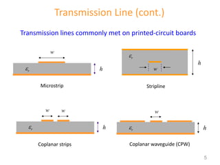
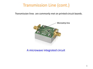
4. Transmission Line (cont.)
CAT 5 cable
(twisted pair)
The two wires of the transmission line are twisted to reduce interference and
radiation from discontinuities.
4

5. Transmission Line (cont.)
Microstrip
h
w
er
er
w
Stripline
h
Transmission lines commonly met on printed-circuit boards
Coplanar strips
h
er
w w
Coplanar waveguide (CPW)
h
er
w
5

6. Transmission Line (cont.)
Transmission lines are commonly met on printed-circuit boards.
A microwave integrated circuit
Microstrip line
6

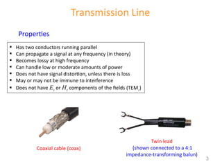
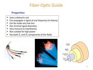
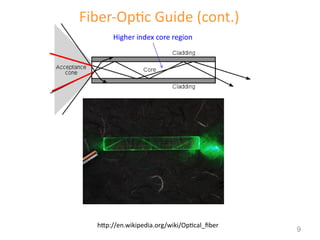
7. Fiber-Optic Guide
Properties
 Uses a dielectric rod
 Can propagate a signal at any frequency (in theory)
 Can be made very low loss
 Has minimal signal distortion
 Very immune to interference
 Not suitable for high power
 Has both Ez and Hz components of the fields
7

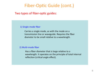
8. Fiber-Optic Guide (cont.)
Two types of fiber-optic guides:
1) Single-mode fiber
2) Multi-mode fiber
Carries a single mode, as with the mode on a
transmission line or waveguide. Requires the fiber
diameter to be small relative to a wavelength.
Has a fiber diameter that is large relative to a
wavelength. It operates on the principle of total internal
reflection (critical angle effect).
8

9. Fiber-Optic Guide (cont.)
http://en.wikipedia.org/wiki/Optical_fiber
Higher index core region
9

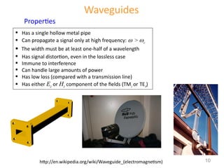
10. Waveguides
 Has a single hollow metal pipe
 Can propagate a signal only at high frequency:  > c
 The width must be at least one-half of a wavelength
 Has signal distortion, even in the lossless case
 Immune to interference
 Can handle large amounts of power
 Has low loss (compared with a transmission line)
 Has either Ez or Hz component of the fields (TMz or TEz)
Properties
http://en.wikipedia.org/wiki/Waveguide_(electromagnetism) 10

11.  Lumped circuits: resistors, capacitors, inductors
neglect time delays (phase)
account for propagation and
time delays (phase change)
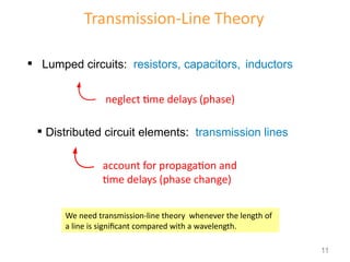
Transmission-Line Theory
 Distributed circuit elements: transmission lines
We need transmission-line theory whenever the length of
a line is significant compared with a wavelength.
11

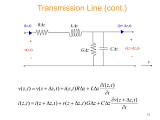
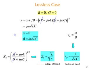
12. Transmission Line
2 conductors
4 per-unit-length parameters:
C = capacitance/length [F/m]
L = inductance/length [H/m]
R = resistance/length [/m]
G = conductance/length [ /m or S/m]

Dz
12

13. Transmission Line (cont.)
z

 
,
i z t
+ + + + + + +
- - - - - - - - - -
 
,
v z t
x x x
B
13
RDz LDz
GDz CDz
z
v(z+z,t)
+
-
v(z,t)
+
-
i(z,t) i(z+z,t)

14. ( , )
( , ) ( , ) ( , )
( , )
( , ) ( , ) ( , )
i z t
v z t v z z t i z t R z L z
t
v z z t
i z t i z z t v z z t G z C z
t

      

  
        

Transmission Line (cont.)
14
RDz LDz
GDz CDz
z
v(z+z,t)
+
-
v(z,t)
+
-
i(z,t) i(z+z,t)

15. Hence
( , ) ( , ) ( , )
( , )
( , ) ( , ) ( , )
( , )
v z z t v z t i z t
Ri z t L
z t
i z z t i z t v z z t
Gv z z t C
z t
   
  
 
     
    
 
Now let Dz  0:
v i
Ri L
z t
i v
Gv C
z t
 
  
 
 
  
 
“Telegrapher’s
Equations”
TEM Transmission Line (cont.)
15

16. To combine these, take the derivative of the first one with
respect to z:
2
2
2
2
v i i
R L
z z z t
i i
R L
z t z
v
R Gv C
t
v v
L G C
t t
   
 
    
   
 
  
 
    
  
 

 
   
 

 
 
 
  
 
 
 
Switch the
order of the
derivatives.
TEM Transmission Line (cont.)
16

17.  
2 2
2 2
( ) 0
v v v
RG v RC LG LC
z t t
  
 
    
 
  
 
The same equation also holds for i.
Hence, we have:
2 2
2 2
v v v v
R Gv C L G C
z t t t
   
   
      
   
   
   
TEM Transmission Line (cont.)
17

18.  
2
2
2
( ) ( ) 0
d V
RG V RC LG j V LC V
dz
 
     
 
2 2
2 2
( ) 0
v v v
RG v RC LG LC
z t t
  
 
    
 
  
 
TEM Transmission Line (cont.)
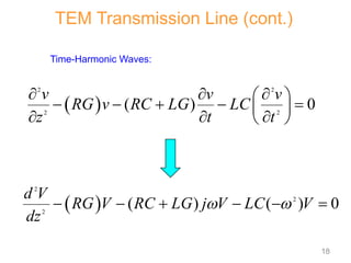
Time-Harmonic Waves:
18

19. Note that
= series impedance/length
   
2
2
2
( )
d V
RG V j RC LG V LC V
dz
 
   
2
( ) ( )( )
RG j RC LG LC R j L G j C
   
     
Z R j L
Y G j C


 
  = parallel admittance/length
Then we can write:
2
2
( )
d V
ZY V
dz

TEM Transmission Line (cont.)
19

20. Let
Convention:
Solution:
2
  ZY
( ) z z
V z Ae Be
 
 
 
 
1/2
( )( )
R j L G j C
  
  
 principal square root
2
2
2
( )
d V
V
dz


Then
TEM Transmission Line (cont.)
 is called the "propagation constant."
/2
j
z z e 

  
  
j
  
 
0, 0
 
 




attenuationcontant
phaseconstant
20

21. TEM Transmission Line (cont.)
0 0
( ) z z j z
V z V e V e e
  
     
 
Forward travelling wave (a wave traveling in the positive z direction):
 
 
 
 
 
0
0
0
( , ) Re
Re
cos
z j z j t
j z j z j t
z
v z t V e e e
V e e e e
V e t z
  
   

  
   
  
 


  
g

0
t 
z
0
z
V e 
 
2
g




2
g
 

The wave “repeats” when:
Hence:
21

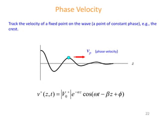
22. Phase Velocity
Track the velocity of a fixed point on the wave (a point of constant phase), e.g., the
crest.
0
( , ) cos( )
z
v z t V e t z

  
  
  
z
vp (phase velocity)
22

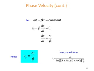
23. Phase Velocity (cont.)
0
constant
 
 


 
 

t z
dz
dt
dz
dt
Set
Hence p
v



 
 
1/2
Im ( )( )
p
v
R j L G j C

 

 
In expanded form:
23

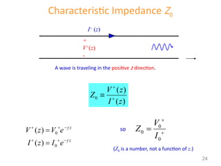
24. Characteristic Impedance Z0
0
( )
( )
V z
Z
I z



0
0
( )
( )
z
z
V z V e
I z I e


  
  


so 0
0
0
V
Z
I



+
V+
(z)
-
I+
(z)
z
A wave is traveling in the positive z direction.
(Z0 is a number, not a function of z.)
24

25. Use Telegrapher’s Equation:
v i
Ri L
z t
 
  
 
so
dV
RI j LI
dz
ZI

  
 
Hence
0 0
z z
V e ZI e
 
    
  
Characteristic Impedance Z0 (cont.)
25

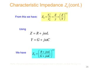
26. From this we have:
Using
We have
1/2
0
0
0
V Z Z
Z
I Y



 
    
 
Y G j C

 
1/2
0
R j L
Z
G j C


 

  

 
Characteristic Impedance Z0 (cont.)
Z R j L

 
Note: The principal branch of the square root is chosen, so that Re (Z0) > 0.
26

27.  
0
0
0 0
j z j j z
z z
z j z
V e e
V z V e V
V e e e
e
e
 
 

  


  

   


 
 
   
 
 
 
0
0 cos
c
, R
os
e j t
z
z
V e t
v z t V z
z
V z
e
e t



 
  

 
 









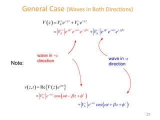
Note:
wave in +z
direction wave in -z
direction
General Case (Waves in Both Directions)
27

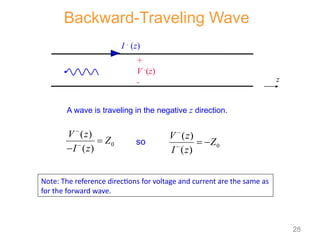
28. Backward-Traveling Wave
0
( )
( )
V z
Z
I z



 0
( )
( )
V z
Z
I z


 
so
+
V -
(z)
-
I -
(z)
z
A wave is traveling in the negative z direction.
Note: The reference directions for voltage and current are the same as
for the forward wave.
28

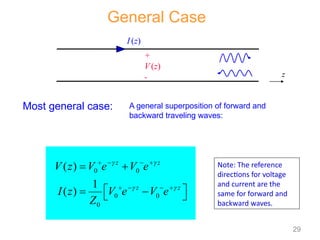
29. General Case
0 0
0 0
0
( )
1
( )
z z
z z
V z V e V e
I z V e V e
Z
 
 
   
   
 
 
 
 
A general superposition of forward and
backward traveling waves:
Most general case:
Note: The reference
directions for voltage
and current are the
same for forward and
backward waves.
29
+
V (z)
-
I (z)
z

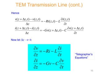
30.  
 
  
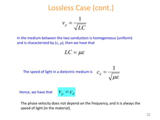
1
2
1
2
0
0 0
0 0
0 0
z z
z z
V z V e V e
V V
I z e e
Z
j R j L G j C
R j L
Z
G j
Z
C
 
 
    


   
 
 

 
   
 
 
 

 






I(z)
V(z)
+
-
z
 
2
m
g




[m/s]
p
v



guided wavelength  g
phase velocity  vp
Summary of Basic TL formulas
30

31. Lossless Case
0, 0
R G
 
 
1/ 2
( )( )
j R j L G j C
j LC
    

    

so 0
LC

 


1/2
0
R j L
Z
G j C


 

  

 
0
L
Z
C

1
p
v
LC

p
v



(indep. of freq.)
(real and indep. of freq.)
31

32. Lossless Case (cont.)
1
p
v
LC

In the medium between the two conductors is homogeneous (uniform)
and is characterized by (, ), then we have that
LC 

The speed of light in a dielectric medium is
1
d
c


Hence, we have that p d
v c

The phase velocity does not depend on the frequency, and it is always the
speed of light (in the material).
(proof given later)
32

33.   0 0
z z
V z V e V e
 
   
 
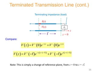
Where do we assign z = 0?
The usual choice is at the load.
I(z)
V(z)
+
-
z
ZL
 z = 0
Terminating impedance (load)
Ampl. of voltage wave
propagating in negative z
direction at z = 0.
Ampl. of voltage wave
propagating in positive z
direction at z = 0.
Terminated Transmission Line
Note: The length l measures distance from the load: z
 

33

34. What if we know
@
V V z
 
 
and
   
0 0
V V V e 
   
   

     
   
z z
V z V e V e
 
  
 
   
 
 
   
0
V V e 
  
  

   
0 0
V V V e
  
    

Terminated Transmission Line (cont.)
  0 0
z z
V z V e V e
 
   
 
Hence
Can we use z = - l as
a reference plane?
I(z)
V(z)
+
-
z
ZL
 z = 0
Terminating impedance (load)
34

35.      
   
( ) ( )
z z
V z V e V e
 
    
 
   
 
 
Terminated Transmission Line (cont.)
     
0 0
z z
V z V e V e
 
   
 
Compare:
Note: This is simply a change of reference plane, from z = 0 to z = -l.
I(z)
V(z)
+
-
z
ZL
 z = 0
Terminating impedance (load)
35

36.   0 0
z z
V z V e V e
 
   
 
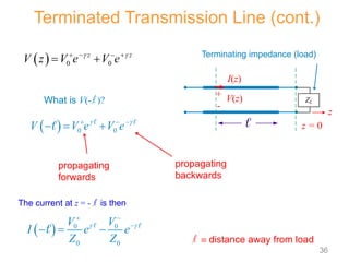
What is V(-l )?
  0 0
V V e V e
 
  
  
 

  0 0
0 0
V V
I e e
Z Z
 
 

  
 

propagating
forwards
propagating
backwards
Terminated Transmission Line (cont.)
l  distance away from load
The current at z = - l is then
I(z)
V(z)
+
-
z
ZL
 z = 0
Terminating impedance (load)
36

37.    
2
0
0
1 L
V
I e e
Z
 


   
 

  2
0
0
0
0 0 1
V
V e
V V e e
e
V
V  
 


 
 

 
 
 

 
 
 
 

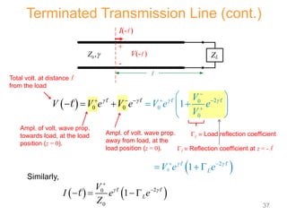
Total volt. at distance l
from the load
Ampl. of volt. wave prop.
towards load, at the load
position (z = 0).
Similarly,
Ampl. of volt. wave prop.
away from load, at the
load position (z = 0).
 
0
2
1 L
V e e
 
 
  
 
L  Load reflection coefficient
Terminated Transmission Line (cont.)
I(-l )
V(-l )
+
l
ZL
-
0,
Z 
l  Reflection coefficient at z = - l
37

38.    
   
 
 
 
2
0
2
2
0
0
2
0
1
1
1
1
L
L
L
L
V V e e
V
I e e
Z
V e
Z Z
I e
 
 


 




   
  
 
    
 
  

 
 









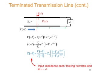
Input impedance seen “looking” towards load
at z = -l .
Terminated Transmission Line (cont.)
I(-l )
V(-l )
+
l
ZL
-
0,
Z 
 
Z 
38

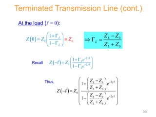
39. At the load (l = 0):
  0
1
0
1
L
L
L
Z Z Z
 
 
  


 
Thus,
 
2
0
0
0
2
0
0
1
1
L
L
L
L
Z Z
e
Z Z
Z Z
Z Z
e
Z Z




 
 


 
 

 
 
 
 
 


 
 
 

 
 



Terminated Transmission Line (cont.)
0
0
L
L
L
Z Z
Z Z

  

 
2
0 2
1
1
L
L
e
Z Z
e




 
 
   

 



Recall
39

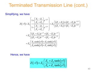
40. Simplifying, we have
 
 
 
0
0
0
tanh
tanh
L
L
Z Z
Z Z
Z Z


 

   
 

 



Terminated Transmission Line (cont.)
 
   
   
   
   
   
   
2
0
2
0 0 0
0 0 2
2 0 0
0
0
0 0
0
0 0
0
0
0
1
1
cosh sinh
cosh sinh
L
L L L
L L
L
L
L L
L L
L
L
Z Z
e
Z Z Z Z Z Z e
Z Z Z
Z Z Z Z e
Z Z
e
Z Z
Z Z e Z Z e
Z
Z Z e Z Z e
Z Z
Z
Z Z




 
 
 
 




 
 
 
 


 
   
   
 
 
    
 
    
 
  

 
 
 

 
 
 
  
  
 
  
 
 

 
 





 
 

 
 



Hence, we have
40

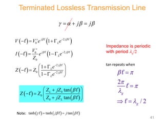
41.    
   
 
2
0
2
0
0
2
0 2
1
1
1
1
j j
L
j j
L
j
L
j
L
V V e e
V
I e e
Z
e
Z Z
e
 
 


 




   
  
 
 
   
 
 
 
 





Impedance is periodic
with period g/2
2
/ 2
g
g
 






 



Terminated Lossless Transmission Line
j j
   
  
Note:      
tanh tanh tan
j j
  
 
  
tan repeats when
 
 
 
0
0
0
tan
tan
L
L
Z jZ
Z Z
Z jZ


 

   
 

 



41

42. For the remainder of our transmission line discussion we will assume that the
transmission line is lossless.
   
   
 
 
 
 
 
2
0
2
0
0
2
0 2
0
0
0
1
1
1
1
tan
tan
j j
L
j j
L
j
L
j
L
L
L
V V e e
V
I e e
Z
V e
Z Z
I e
Z jZ
Z
Z jZ
 
 




 




   
  
  
 
    
 
 
 

  
 

 
 
 









0
0
2
L
L
L
g
p
Z Z
Z Z
v






 



Terminated Lossless Transmission Line
I(-l )
V(-l )
+
l
ZL
-
0 ,
Z 
 
Z 
42

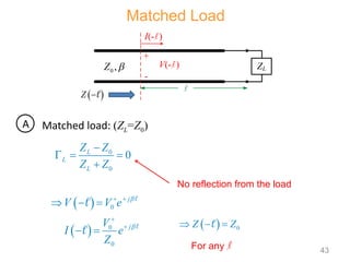
43. Matched load: (ZL=Z0)
0
0
0
L
L
L
Z Z
Z Z

  

For any l
No reflection from the load
A
Matched Load
I(-l )
V(-l )
+
l
ZL
-
0 ,
Z 
 
Z 
  0
Z Z
  

 
 
0
0
0
j
j
V V e
V
I e
Z


 


  
 




43

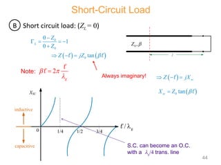
44. Short circuit load: (ZL = 0)
   
0
0
0
0
1
0
tan
L
Z
Z
Z jZ 

   

  
 
Always imaginary!
Note:
B
2
g
 




  sc
Z jX
  

S.C. can become an O.C.
with a g/4 trans. line
0 1/4 1/2 3/4
g
/ 

XSC
inductive
capacitive
Short-Circuit Load
l
0 ,
Z 
 
0 tan
sc
X Z 
 
44

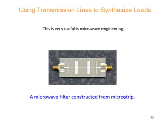
45. Using Transmission Lines to Synthesize Loads
A microwave filter constructed from microstrip.
This is very useful is microwave engineering.
45

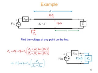
46.  
 
 
0
0
0
tan
tan
L
in
L
Z jZ d
Z Z d Z
Z jZ d


 

    
 

 
  in
TH
in TH
Z
V d V
Z Z
 
    

 
I(-l)
V(-l)
+
l
ZL
-
0
Z 

ZTH
VTH
d
Zin
+
-
ZTH
VTH
+
Zin
V(-d)
+
-
Example
Find the voltage at any point on the line.
46

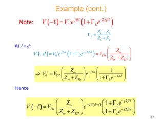
47. Note:    
0
2
1 j
L
j
V V e e
 
 
 

  

0
0
L
L
L
Z Z
Z Z

 

   
2
0 1
j d j d in
TH
in TH
L
V d
Z
Z
e V
Z
V e  
 
   
 
  

 
   
2
2
1
1
j
j d
in L
TH j d
m TH L
Z e
V V e
Z Z e




 

   
 
     
  
 
 



At l = d :
Hence
Example (cont.)
0 2
1
1
j d
in
TH j d
in TH L
Z
V V e
Z Z e


 

   
     
  
 
 
47

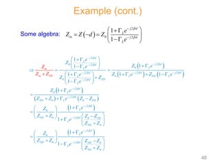
48. Some algebra:  
2
0 2
1
1
j d
L
in j d
L
e
Z Z d Z
e




 
 
    

 
 
   
 
   
 
2
2
0 2
0
2 2
2
0
0 2
2
0
2
0 0
2
0
2
0 0
0
1
1
1
1 1
1
1
1
1
1
j d
L
j d
j d
L
L
j d j d
j d
L TH L
L
TH
j d
L
j d
L
j d
TH L TH
j d
L
j d
TH TH
L
TH
in
in TH
e
Z
Z e
e
Z e Z e
e
Z Z
e
Z e
Z Z e Z Z
e
Z
Z
Z
Z Z
Z Z Z
e
Z Z
Z



 









 






 
 
   
 
 
  
      
 

 
 
 
 

  


 
 
  
  

     

 

 
2
0
2
0 0
0
1
1
j d
L
j d
TH TH
L
TH
e
Z Z Z Z
e
Z Z




 
 
 
  

     

 
Example (cont.)
48

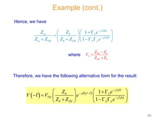
49.    
2
0
2
0
1
1
j
j d L
TH j d
TH S L
Z e
V V e
Z Z e




 

   
 
     
   
   



2
0
2
0
1
1
j d
in L
j d
in TH TH S L
Z Z e
Z Z Z Z e




  
 
   
    
  
where 0
0
TH
S
TH
Z Z
Z Z

 

Example (cont.)
Therefore, we have the following alternative form for the result:
Hence, we have
49

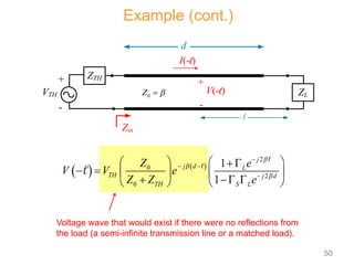
50.    
2
0
2
0
1
1
j
j d L
TH j d
TH S L
Z e
V V e
Z Z e




 

   
 
     
   
   



Example (cont.)
I(-l)
V(-l)
+
l
ZL
-
0
Z 

ZTH
VTH
d
Zin
+
-
Voltage wave that would exist if there were no reflections from
the load (a semi-infinite transmission line or a matched load).
50

51.  
 
       
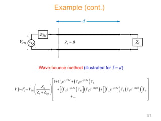
2 2
2 2 2 2
0
0
1 j d j d
L L S
j d j d j d j d
TH L S L L S L S
TH
e e
Z
V d V e e e e
Z Z
 
   
 
   
 
    
 
  
   
          
     
 

 
 

 

Example (cont.)
ZL
0
Z 

ZTH
VTH
d
+
-
Wave-bounce method (illustrated for l = d):
51

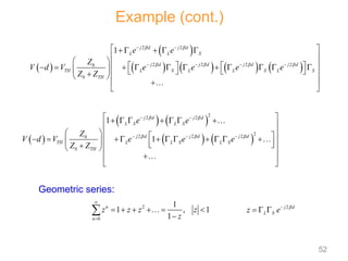
52. Example (cont.)
 
   
   
2
2 2
2
2 2 2
0
0
1
1
j d j d
L S L S
j d j d j d
TH L L S L S
TH
e e
Z
V d V e e e
Z Z
 
  
 
  
 
      
 
  
 
          
  
 
 

  

 
 



Geometric series:
2
0
1
1 , 1
1
n
n
z z z z
z


     

 
 
 
       
2 2
2 2 2 2
0
0
1 j d j d
L L S
j d j d j d j d
TH L S L L S L S
TH
e e
Z
V d V e e e e
Z Z
 
   
 
   
 
    
 
  
   
          
     
 

 
 

 

2
j d
L S
z e 

  
52

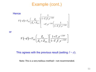
53. Example (cont.)
or
 
2
0
2
0
2
1
1
1
1
j d
L s
TH
j d
TH
L j d
L s
e
Z
V d V
Z Z
e
e






 
 
 
  
    
 

   
 
 
 
 
 
 
 
2
0
2
0
1
1
j d
L
TH j d
TH L s
Z e
V d V
Z Z e




  
 
    
  
  
This agrees with the previous result (setting l = d).
Note: This is a very tedious method – not recommended.
Hence
53

54. I(-l)
V(-l)
+
l
ZL
-
0 ,
Z 
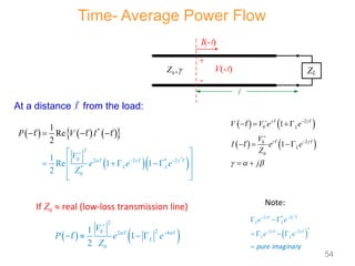
At a distance l from the load:
     
 
  
*
*
2
0 2 2 * 2
*
0
1
Re 1 1
1
R
2
e
2
L L
V
e e
Z
V I
e
P
  

 
 
 
 
   
 
 
 
  
  
   
2
2
0 2 4
0
1
1
2
L
V
P e e
Z
 


   
 

If Z0  real (low-loss transmission line)
Time- Average Power Flow
   
   
2
0
2
0
0
1
1
L
L
V V e e
V
I e e
Z
j
 
 
  
 


   
  
 
 
 


 
*
2 * 2
*
2 2
L L
L L
e e
e e
 
 
 
 
 
   

 
 
pure imaginary
Note:
54

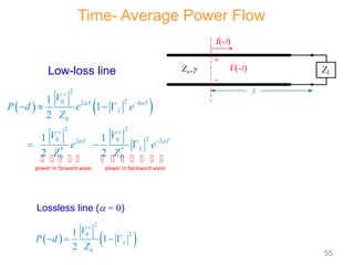
55. Low-loss line
   
2
2
0 2 4
0
2 2
2
0 0
2 2
* *
0 0
1
1
2
1 1
2 2
L
L
V
P d e e
Z
V V
e e
Z Z
 
 


 

   
  
 
 
           
power in forward wave power in backward wave
   
2
2
0
0
1
1
2
L
V
P d
Z

   
Lossless line ( = 0)
Time- Average Power Flow
I(-l)
V(-l)
+
l
ZL
-
0 ,
Z 
55

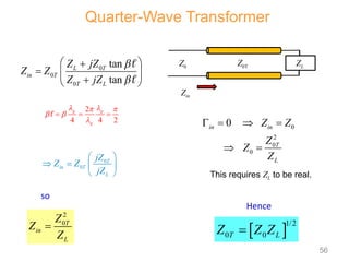
56. 0
0
0
tan
tan
L T
in T
T L
Z jZ
Z Z
Z jZ


 

  

 


2
4 4 2
g g
g
 
 
 

  

0
0
T
in T
L
jZ
Z Z
jZ
 
   
 
0
2
0
0
0
in in
T
L
Z Z
Z
Z
Z
   
 
Quarter-Wave Transformer
2
0T
in
L
Z
Z
Z

so
 
1/2
0 0
T L
Z Z Z

Hence
This requires ZL to be real.
ZL
Z0 Z0T
Zin
56

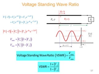
57.   2
0 1 L
j j
L
V V e e
 
 
    

   
 
2
0
2
0
1
1 L
j j
L
j
j j
L
V V e e
V e e e
 

 
 
 
   
  
 
 

 
 
max 0
min 0
1
1
L
L
V V
V V


  
  
  max
min
V
V

VoltageStanding WaveRatio VSWR
Voltage Standing Wave Ratio
I(-l )
V(-l )
+
l
ZL
-
0 ,
Z 
1
1
L
L
 

 
VSWR
z
1+ L

1
1- L

0
( )
V z
V 
/ 2
z 
 
0
z 
57

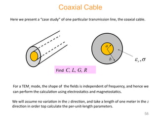
58. Coaxial Cable
Here we present a “case study” of one particular transmission line, the coaxial cable.
a
b ,
r
 
Find C, L, G, R
We will assume no variation in the z direction, and take a length of one meter in the z
direction in order top calculate the per-unit-length parameters.
58
For a TEMz mode, the shape of the fields is independent of frequency, and hence we
can perform the calculation using electrostatics and magnetostatics.

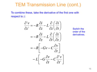
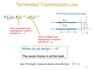
59. Coaxial Cable (cont.)
-l0
l0
a
b
r

0 0
0
ˆ ˆ
2 2 r
E
 
 
    
 
 
   
 
   
 
Find C (capacitance / length)
Coaxial cable
h = 1 [m]
r

From Gauss’s law:
0
0
ln
2
B
AB
A
b
r
a
V V E dr
b
E d
a



 
  
 
   
 

 
59

60. -l0
l0
a
b
r

Coaxial cable
h = 1 [m]
r

 
0
0
0
1
ln
2 r
Q
C
V b
a


 
 
   
   
 
 


Hence
We then have
0
F/m
2
[ ]
ln
r
C
b
a
 

 
 
 
Coaxial Cable (cont.)
60

61. ˆ
2
I
H 
 
 
  
 
Find L (inductance / length)
From Ampere’s law:
Coaxial cable
h = 1 [m]
r

I
0
ˆ
2
r
I
B   
 
 
  
 
(1)
b
a
B d

 
 
S
h
I
I
z
center conductor
Magnetic flux:
Coaxial Cable (cont.)
61
Note: We ignore “internal inductance”
here, and only look at the magnetic field
between the two conductors (accurate
for high frequency.

62. Coaxial cable
h = 1 [m]
r

I
  0
0
0
1
2
ln
2
b
r
a
b
r
a
r
H d
I
d
I b
a

   
  

 



 
  
 


0
1
ln
2
r
b
L
I a

 

 
   
 
0
H/m
ln [ ]
2
r b
L
a
 

 
  
 
Hence
Coaxial Cable (cont.)
62

63. 0
H/m
ln [ ]
2
r b
L
a
 

 
  
 
Observation:
0
F/m
2
[ ]
ln
r
C
b
a
 

 
 
 
 
0 0 r r
LC     
 
This result actually holds for any transmission line.
Coaxial Cable (cont.)
63

64. 0
H/m
ln [ ]
2
r b
L
a
 

 
  
 
For a lossless cable:
0
F/m
2
[ ]
ln
r
C
b
a
 

 
 
 
0
L
Z
C

0 0
1
ln [ ]
2
r
r
b
Z
a


 
 
 
 
 
0
0
0
376.7303 [ ]



  
Coaxial Cable (cont.)
64

65. -l0
l0
a
b

0 0
0
ˆ ˆ
2 2 r
E
 
 
    
 
 
   
 
   
 
Find G (conductance / length)
Coaxial cable
h = 1 [m]

From Gauss’s law:
0
0
ln
2
B
AB
A
b
r
a
V V E dr
b
E d
a



 
  
 
   
 

 
Coaxial Cable (cont.)
65

66. -l0
l0
a
b
 J E


We then have leak
I
G
V

 
0
0
(1)2
2
2
2
leak a
a
r
I J a
a E
a
a
 
 

 

 
 




 
  
 

0
0
0
0
2
2
ln
2
r
r
a
a
G
b
a

 
 

 
 
 
 

 
 
 


2
[S/m]
ln
G
b
a


 
 
 
or
Coaxial Cable (cont.)
66

67. Observation:
F/m
2
[ ]
ln
C
b
a


 
 
 
G C


 
  
 
This result actually holds for any transmission line.
2
[S/m]
ln
G
b
a


 
 
 
0 r
  

Coaxial Cable (cont.)
67

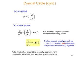
68. G C


 
  
 
To be more general:
tan
G
C


 
 
 
 
 
tan
G
C



Note: It is the loss tangent that is usually (approximately)
constant for a material, over a wide range of frequencies.
Coaxial Cable (cont.)
As just derived,
The loss tangent actually arises from
both conductivity loss and polarization
loss (molecular friction loss), ingeneral.
68
This is the loss tangent that would
arise from conductivity effects.

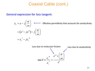
69. General expression for loss tangent:
 
c
c c
j
j j
j

 


 

 
 
   
 
 
 
    
 
 
 
tan c
c


 



 
  
  
 


Effective permittivity that accounts for conductivity
Loss due to molecular friction Loss due to conductivity
Coaxial Cable (cont.)
69

70. Find R (resistance / length)
Coaxial cable
h = 1 [m]
Coaxial Cable (cont.)
,
b rb
 
a
b

,
a ra
 
a b
R R R
 
1
2
a sa
R R
a

 
  
 
1
2
b sb
R R
b

 
  
 
1
sa
a a
R
 

1
sb
b b
R
 

0
2
a
ra a

  

0
2
b
rb b

  

Rs = surface resistance of metal
70

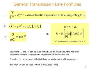
71. General Transmission Line Formulas
tan
G
C



 
0 0 r r
LC     
 
 
0
lossless
L
Z
C
  characteristic impedance of line (neglectingloss)
(1)
(2)
(3)
Equations (1) and (2) can be used to find L and C if we know the material
properties and the characteristic impedance of the lossless line.
Equation (3) can be used to find G if we know the material loss tangent.
a b
R R R
 
tan
G
C



(4)
Equation (4) can be used to find R (discussed later).
,
i
C i a b
 
contour of conductor,
2
2
1
( )
i
i s sz
C
R R J l dl
I
 
  
 
 


71

72. General Transmission Line Formulas (cont.)
 tan
G C
 

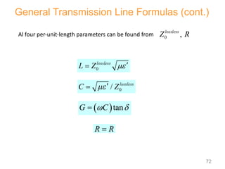
0
lossless
L Z 

0
/ lossless
C Z


R R

Al four per-unit-length parameters can be found from 0 ,
lossless
Z R
72

73. Common Transmission Lines
0 0
1
ln [ ]
2
lossless r
r
b
Z
a


 
 
 
 
 
Coax
Twin-lead
1
0
0 cosh [ ]
2
lossless r
r
h
Z
a
 
 
  
 
 
 
2
1 2
1
2
s
h
a
R R
a h
a

 
 
 
 
 
 
  
 
 

 
 
 
 
1 1
2 2
sa sb
R R R
a b
 
   
 
   
   
a
b
,
r r
 
h
,
r r
 
a a
73

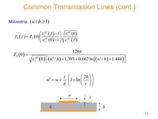
74. Common Transmission Lines (cont.)
Microstrip
   
 
 
 
 
0 0
1 0
0
0 1
eff eff
r r
eff eff
r r
f
Z f Z
f
 
 
 

  
 

 
 
     
 
0
120
0
0 / 1.393 0.667ln / 1.444
eff
r
Z
w h w h



 
 
  
 
( / 1)
w h 
2
1 ln
t h
w w
t

 
 
     
 
 
 
h
w
er
t
74

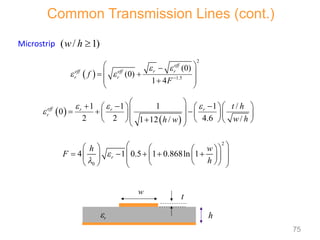
75. Common Transmission Lines (cont.)
Microstrip ( / 1)
w h 
h
w
er
t
 
2
1.5
(0)
(0)
1 4
eff
r r
eff eff
r r
f
F
 
  
 

 
 
 

 
 
 
1 1 1
1 /
0
2 2 4.6 /
1 12 /
eff r r r
r
t h
w h
h w
  

 
    
   
 
  
    
 
   
  
 
2
0
4 1 0.5 1 0.868ln 1
r
h w
F
h


 
   
 
    
 
   
 
 
 
 
   
75

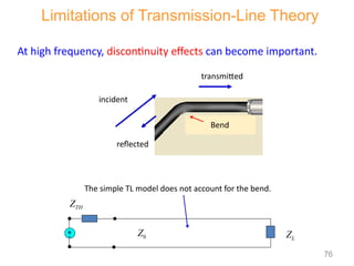
76. At high frequency, discontinuity effects can become important.
Limitations of Transmission-Line Theory
Bend
incident
reflected
transmitted
The simple TL model does not account for the bend.
ZTH
ZL
Z0
+
-
76

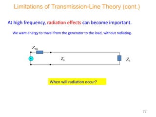
77. At high frequency, radiation effects can become important.
When will radiation occur?
We want energy to travel from the generator to the load, without radiating.
Limitations of Transmission-Line Theory (cont.)
ZTH
ZL
Z0
+
-
77

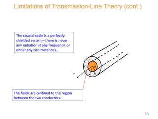
78. r
 a
b
z
The coaxial cable is a perfectly
shielded system – there is never
any radiation at any frequency, or
under any circumstances.
The fields are confined to the region
between the two conductors.
Limitations of Transmission-Line Theory (cont.)
78

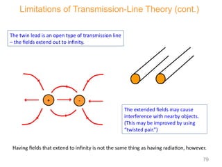
79. The twin lead is an open type of transmission line
– the fields extend out to infinity.
The extended fields may cause
interference with nearby objects.
(This may be improved by using
“twisted pair.”)
+ -
Limitations of Transmission-Line Theory (cont.)
Having fields that extend to infinity is not the same thing as having radiation, however.
79

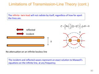
80. The infinite twin lead will not radiate by itself, regardless of how far apart
the lines are.
h
incident
reflected
The incident and reflected waves represent an exact solution to Maxwell’s
equations on the infinite line, at any frequency.
 
*
1
ˆ
Re E H 0
2
t
S
P dS

 
   
 
 

S
+ -
Limitations of Transmission-Line Theory (cont.)
No attenuation on an infinite lossless line
80

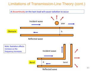
81. A discontinuity on the twin lead will cause radiation to occur.
Note: Radiation effects
increase as the
frequency increases.
Limitations of Transmission-Line Theory (cont.)
h
Incident wave
pipe
Obstacle
Reflected wave
Bend h
Incident wave
bend
Reflected wave
81

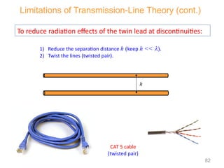
82. To reduce radiation effects of the twin lead at discontinuities:
h
1) Reduce the separation distance h (keep h << ).
2) Twist the lines (twisted pair).
Limitations of Transmission-Line Theory (cont.)
CAT 5 cable
(twisted pair)
82