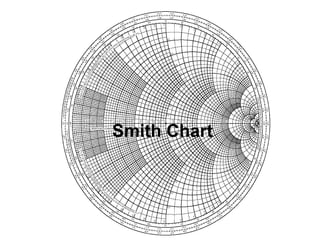
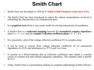
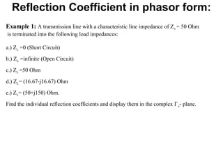
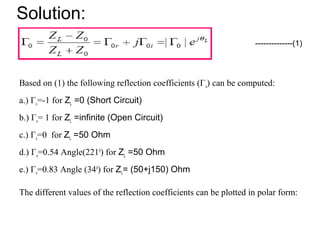
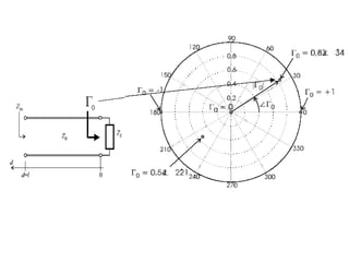
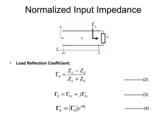
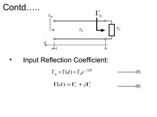
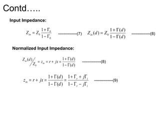
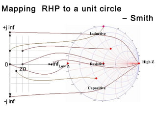
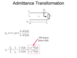
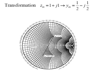
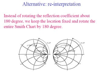
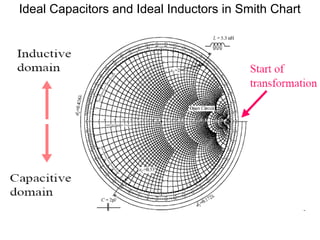
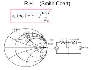
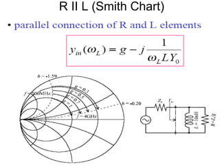
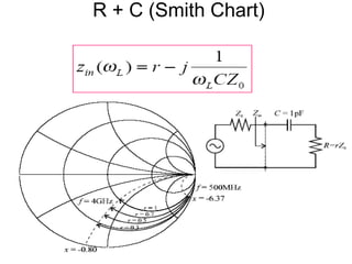
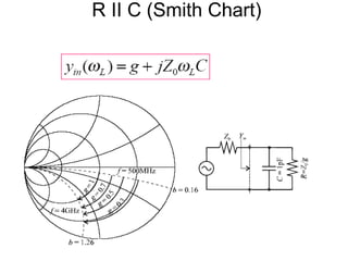
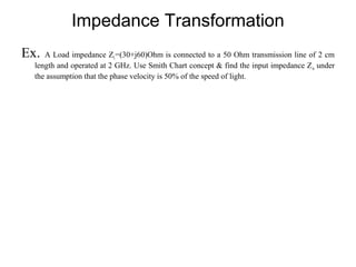
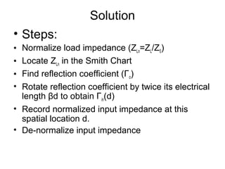
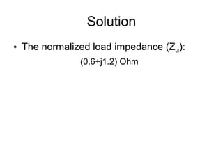
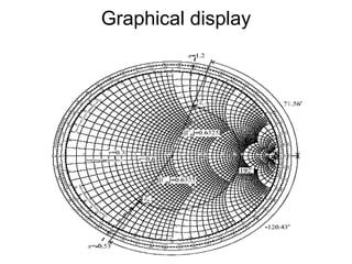
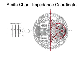
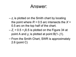
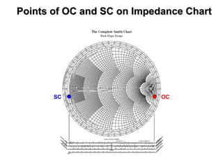
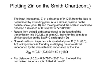
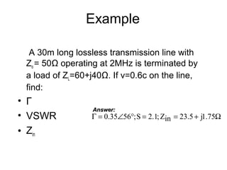
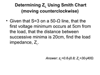
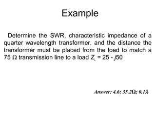
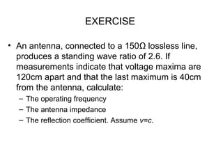
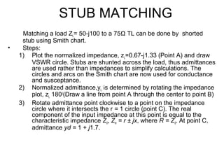
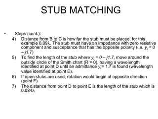
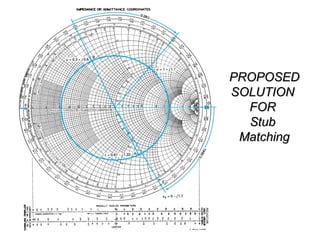
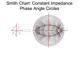
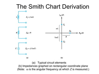
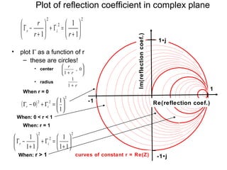
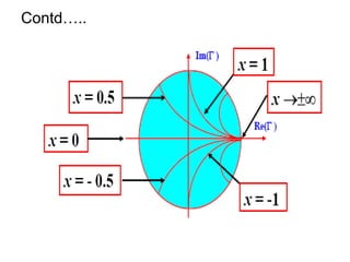
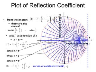
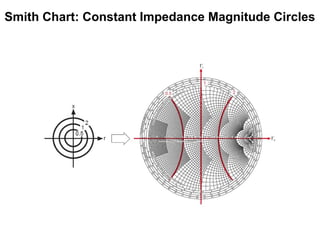
The document discusses the Smith chart, which is a graphical tool used to solve transmission line problems. Some key points: - The Smith chart was developed in 1939 and allows tedious transmission line calculations to be done graphically. - It provides a mapping between the normalized impedance plane and the reflection coefficient plane. Circles of constant resistance and reactance are plotted, along with the reflection coefficient. 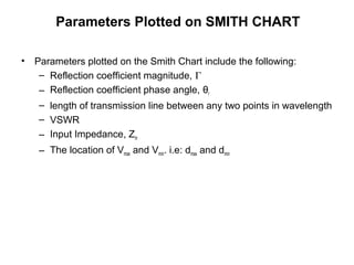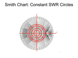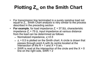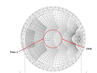- Parameters like impedance, admittance, reflection coefficient, VSWR can all be plotted and derived from locations on the chart. 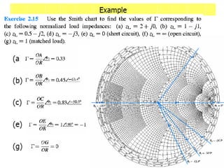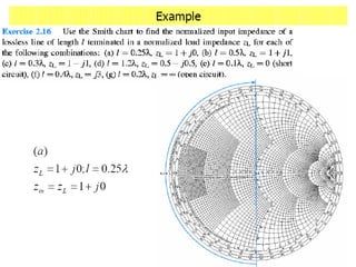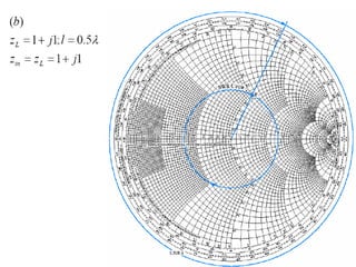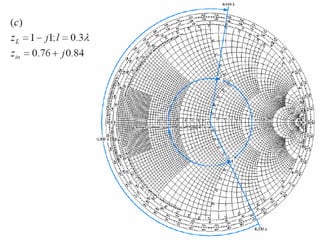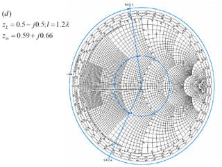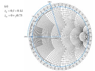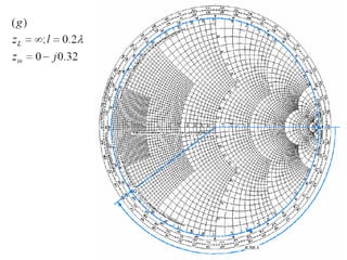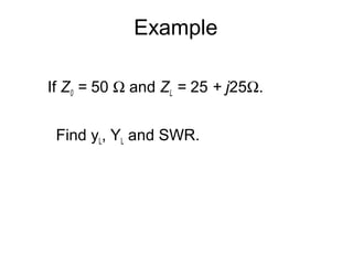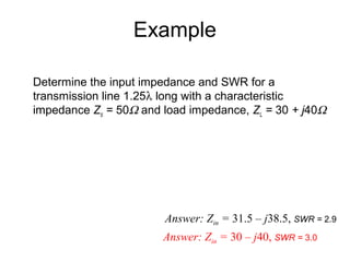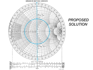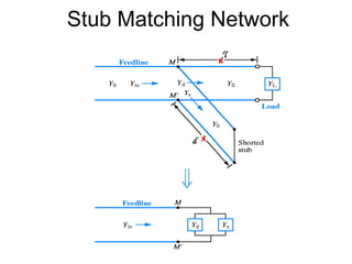- Examples are given of using the Smith chart to determine input impedance, reflection coefficient, and stub matching of transmission lines with various termination impedances.

1. Smith Chart
------A Graphical Representation
By
Dr . Taimoor Khan

2. Smith Chart

3. Smith Chart
• Smith Chart was developed in 1939 by P. Smith at Bell Telephone Laboratory USA.
• The Smith Chart has been introduced to reduce the tedious manipulations involved in
calculating the characteristics of a transmission lines.
• It is graphical tool which is very much useful for solving transmission line problems.
• A Smith Chart is a conformal mapping between the normalized complex impedance
plane ( z = r + j x ) and the complex reflection coefficient plane ( Γ= Γr+ jΓi).
• It is essentially a plot of the voltage reflection coefficient (Γ) in complex plane.
• It can be used to convert from voltage reflection coefficient (Γ) to normalized
impedances (z=Z/Z0) and admittances (y=Y/Y0),and vice versa.
• It consists of a Polar/Cartesian plot of reflection coefficient onto which is overlaid
circles of constant real and constant imaginary impedance. The standard chart is plotted
for Γ≤1.
• Today, Smith Chart is a presentation medium in computer-aided design (CAD) software.

4. • Parameters plotted on the Smith Chart include the following:
– Reflection coefficient magnitude, Γ
– Reflection coefficient phase angle, θr
– length of transmission line between any two points in wavelength
– VSWR
– Input Impedance, Zin
– The location of Vmax and Vmin. i.e: dmax and dmin
Parameters Plotted on SMITH CHART

5. (a) Typical circuit elements
(b) Impedances graphed on rectangular coordinate plane
(Note: ω is the angular frequency at which Z is measured.)
The Smith Chart Derivation

6. Reflection Coefficient in phasor form:
Example 1: A transmission line with a characteristic line impedance of Zo = 50 Ohm
is terminated into the following load impedances:
a.) ZL =0 (Short Circuit)
b.) ZL =infinite (Open Circuit)
c.) ZL =50 Ohm
d.) ZL= (16.67-j16.67) Ohm
e.) ZL= (50+j150) Ohm.
Find the individual reflection coefficients and display them in the complex Γo- plane.

7. Solution:
Based on (1) the following reflection coefficients (Γo) can be computed:
a.) Γo=-1 for ZL =0 (Short Circuit)
b.) Γo= 1 for ZL =infinite (Open Circuit)
c.) Γo=0 for ZL =50 Ohm
d.) Γo=0.54 Angle(2210
) for ZL =50 Ohm
e.) Γo=0.83 Angle (340
) for ZL= (50+j150) Ohm
The different values of the reflection coefficients can be plotted in polar form:
--------------(1)

9. Normalized Input Impedance
• Load Reflection Coefficient:
0
0
0
ZZ
ZZ
L
L
+
−
=Γ
--------------(2)
ir j 000 Γ+Γ=Γ --------------(3)
Li
e θ
00 Γ=Γ --------------(4)

10. Contd…..
• Input Reflection Coefficient:
lj
in ed β2
0)( −
Γ=Γ=Γ
ir jd Γ+Γ=Γ )(
--------------(5)
--------------(6)

11. Input Impedance:
Contd…..
--------------(7)
0
0
0
1
1
Γ−
Γ+
= ZZin
Normalized Input Impedance:
)(1
)(1
)( 0
d
d
ZdZin
Γ−
Γ+
= --------------(8)
)(1
)(1)(
0 d
d
jxrz
Z
dZ
in
in
Γ−
Γ+
=+== --------------(8)
ir
ir
in
j
j
d
d
jxrz
Γ−Γ−
Γ+Γ+
=
Γ−
Γ+
=+=
1
1
)(1
)(1
--------------(9)

12. Contd…..
)1(
)1(
)1(
)1(
ir
ir
ir
ir
in
j
j
j
j
jxrz
Γ+Γ−
Γ+Γ−
Γ−Γ−
Γ+Γ+
=+= --------------(10)
Real Part:
--------------(11)
--------------(12)
Imaginary Part:

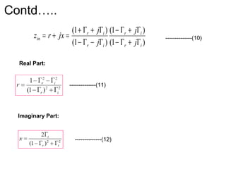
13. ( )[ ] 2222
11 irirr Γ−Γ−=Γ+Γ−
From (11)
----------------- (13)
2
2
2
1
1
1






+
=Γ+





+
−Γ
rr
r
ir ----------------- (14)
( ) ( )222
)( cba ir =−Γ+−Γ ----------------- (15)
Resistive Circle , r-circle

14. Contd….

15. Plot of reflection coefficient in complex plane
-1
1
Re(reflection coef.)
Im(reflectioncoef.)
1•j
-1•jcurves of constant r = Re(Z)
• plot Γ as a function of r
– these are circles!
When: r = 1
When: 0 < r < 1
When: r > 1
When r = 0
• radius






+
0,
1 r
r
r+1
1
• center
2
2
2
1
1
1






+
=Γ+





+
−Γ
rr
r
ir
( )
2
22
1
1
0 





=Γ+−Γ ir
2
2
2
11
1
11
1






+
=Γ+





+
−Γ ir

16. ( )[ ] iirx Γ=Γ+Γ− 21
22
From (12)
----------------- (16)
( )
22
2 11
1 





=





−Γ+−Γ
xx
ir
----------------- (17)
( ) ( )222
)( cba ir =−Γ+−Γ ----------------- (18)
Reactance Circle, x-circle

17. Contd…..

18. Plot of Reflection Coefficient
-1
1
Re(reflection coef.)
Im(reflectioncoef.)
j
-j
• plot Γ as a function of x
– x = ± ∞
When: x < 0
When: x > 0
When: x = 0
• from the Im part:
( ) 2
2
2
0
1
0
1
1 =





−Γ+−Γ ir
( )
∞
=





∞±
−Γ+−Γ
11
1
2
2
ir
curves of constant x = Im(Z)
– these are also
circles!
• radius





x
1
,1
x
1
• center
( )
22
2 11
1 





=





−Γ+−Γ
xx
ir

19. Mapping RHP to a unit circle
– Smith
Chart
Inductive
Resistive
Low Z
High Z
Capacitive

20. Admittance Transformation

23. Ideal Capacitors and Ideal Inductors in Smith Chart

24. R +L (Smith Chart)

25. R II L (Smith Chart)

26. R + C (Smith Chart)

27. R II C (Smith Chart)

28. Impedance Transformation
Ex. A Load impedance ZL=(30+j60)Ohm is connected to a 50 Ohm transmission line of 2 cm
length and operated at 2 GHz. Use Smith Chart concept & find the input impedance Zin under
the assumption that the phase velocity is 50% of the speed of light.

29. Solution
• Steps:
• Normalize load impedance (ZLn=ZL/Z0)
• Locate ZLn in the Smith Chart
• Find reflection coefficient (Γo)
• Rotate reflection coefficient by twice its electrical
length βd to obtain Γin(d)
• Record normalized input impedance at this
spatial location d.
• De-normalize input impedance

30. Solution
• The normalized load impedance (ZLn):
(0.6+j1.2) Ohm

31. Graphical display

39. Smith Chart: Impedance Coordinate

40. Smith Chart: Admittance Coordinate

41. Smith Chart: Constant SWR Circles

42. Plotting SWR circle on the Smith Chart
– Any lossless line can be represented on the Smith chart
by a circle having its origin at 1± j0 (center of the chart)
and radius equal to the distance between the origin and
the impedance plot.
– Therefore, SWR corresponding to any particular circle isSWR corresponding to any particular circle is
equal to the value of Zequal to the value of ZLL /Z/Z00 at which the circle crosses theat which the circle crosses the
horizontal axis on the right side of the chart.horizontal axis on the right side of the chart.

43. If Z0 = 50 Ω and ZL = 25 + j25Ω.
Find yL, YL and SWR.
Example

44. Answer:
– zL is plotted on the Smith chart by locating
the point where R = 0.5 arc intersects the X =
0.5 arc on the top half of the chart.
– ZL = 0.5 + j0.5 is plotted on the Figure 34 at
point A and yL is plotted at point B(1- j1).
– From the Smith Chart, SWR is approximately
2.6 (point C)

45. PROPOSEDPROPOSED
SOLUTIONSOLUTION
FORFOR
ExampleExample

46. SC and OC points on the Smith chartSC and OC points on the Smith chart
• The location of SC and OC points are
different depending on Impedance or
Admittance chart.

47. Points of OC and SC on Impedance ChartPoints of OC and SC on Impedance Chart
SC OC

48. Points of OC and SC on Admittance ChartPoints of OC and SC on Admittance Chart
OC SC

49. Smith Chart: Constant Impedance Magnitude Circles

50. • For transmission line terminated in a purely resistive load not
equal to Z0 , Smith Chart analysis is very similar to the process
described in the preceding section
• For example, for load impedance ZL = 37.5Ω, characteristic
impedance Z0 = 75 Ω, input impedance at various distance
from the load can be determined as follows
– Normalized impedance, zL=0.5
– zL = 0.5 is plotted on the Smith chart. A circle is drawn that
passes through point A with its centre located at the
intersection of the R = 1 and X = 0 arc.
– SWR is read at the intersection of the circle and the X = 0
line on the right side, SWR = 2
Plotting Zin on the Smith Chart

51. SWR
Point A

52. – The input impedance, Zin at a distance of 0.125λ from the load is
determined by extending point A to a similar position on the
outside scale (point B) and moving around the scale in clockwise
direction a distance of 0.125λ=0.127x720°=90°
– Rotate from point B a distance equal to the length of the
transmission line ( 0.125λ at point C). Transfer this point to a
similar position on the SWR=2 circle (point D)
– Normalized input impedance is located at point D (0.8 +j0.6).
Actual impedance is found by multiplying the normalized
impedance by the characteristic impedance of the line
– For distance of 0.3λ= 0.3x720°= 216° from the load, the
normalized impedance is plotted at point E
Plotting Zin on the Smith Chart(cont.)
Ω+=+= 45j6075)6.0j8.0(inZ

54. Example
Determine the input impedance and SWR for a
transmission line 1.25λ long with a characteristic
impedance Zo = 50Ω and load impedance, ZL = 30 + j40Ω
Answer: Zin = 31.5 – j38.5, SWR = 2.9
Answer: Zin = 30 – j40, SWR = 3.0

55. PROPOSEDPROPOSED
SOLUTIONSOLUTION

56. Example
A 30m long lossless transmission line with
Zo = 50Ω operating at 2MHz is terminated by
a load of ZL=60+j40Ω. If v=0.6c on the line,
find:
• Γ
• VSWR
• Zin
Ω+==°∠=Γ 75.1j5.23inZ;1.2S;5635.0
Answer:Answer:

57. Vmax
versus
Vmin

58. Determining ZL Using Smith Chart
(moving counterclockwise)
• Given that S=3 on a 50-Ω line, that the
first voltage minimum occurs at 5cm from
the load, that the distance between
successive minima is 20cm, find the load
impedance, ZL.
Answer: zAnswer: zLL=0.6-j0.8; Z=0.6-j0.8; ZLL=30-j40=30-j40ΩΩ

59. Example
Determine the SWR, characteristic impedance of a
quarter wavelength transformer, and the distance the
transformer must be placed from the load to match a
75 Ω transmission line to a load ZL = 25 - j50
Answer: 4.6; 35.2Ω; 0.1λ

60. EXERCISE
• An antenna, connected to a 150Ω lossless line,
produces a standing wave ratio of 2.6. If
measurements indicate that voltage maxima are
120cm apart and that the last maximum is 40cm
from the antenna, calculate:
– The operating frequency
– The antenna impedance
– The reflection coefficient. Assume v=c.

61. STUB MATCHING
Matching a load ZL= 50-j100 to a 75Ω TL can be done by shorted
stub using Smith chart.
• Steps:
1) Plot the normalized impedance, zL=0.67-j1.33 (Point A) and draw
VSWR circle. Stubs are shunted across the load, thus admittances
are used rather than impedances to simplify calculations. The
circles and arcs on the Smith chart are now used for conductance
and susceptance.
2) Normalized admittance,yL is determined by rotating the impedance
plot, zL 180o
(Draw a line from point A through the center to point B)
3) Rotate admittance point clockwise to a point on the impedance
circle where it intersects the r = 1 circle (point C). The real
component of the input impedance at this point is equal to the
characteristic impedance Z0, Zin = r ± jx, where R = Z0. At point C,
admittance yd = 1 + j1.7.

62. STUB MATCHING
• Steps (cont.):
4) Distance from B to C is how far the stub must be placed, for this
example 0.09λ. The stub must have an impedance with zero resistive
component and susceptance that has the opposite polarity (i.e. ys = 0
– j1.7)
5) To find the length of the stub where ys = 0 – j1.7, move around the
outside circle of the Smith chart (R = 0), having a wavelength
identified at point D until an admittance ys = 1.7 is found (wavelength
value identified at point E).
6) If open stubs are used, rotation would begin at opposite direction
(point F)
7) The distance from point D to point E is the length of the stub which is
0.084λ

63. PROPOSEDPROPOSED
SOLUTIONSOLUTION
FORFOR
StubStub
MatchingMatching

64. Example
For a transmission line with a characteristic
impedance Z0 = 300Ω and a load with
complex impedance ZL = 450 + j600,
determine:
SWR,
the distance a shorted stub must be placed from
the load to match the load to the line
the length of the stub.

65. 2BdAd λ=+
Note that:
 In this case, we have two possible shunted stubs.
To avoid confusion, we normally choose to match the shorter stub
and one at a position closer to the load  lA and dA
yd. lB and dB is the
alternative stub
distance and stub
length

66. Stub Matching Network
l
x
xd
l
x
xd

67. Smith Chart: Constant Impedance
Phase Angle Circles

68. Few Other Applications
• Unary Operators
• Squares a2
• square roots
• tangents tan q
• cotangents cot q
• inverse tangents tan-1 a
• Inverse cotangents cot-1 a
• Binary Operators
• multiplication  a • b
• Division c/a
• geometric mean

69. Please Study for your Mid Sem 1!