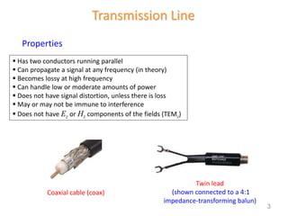
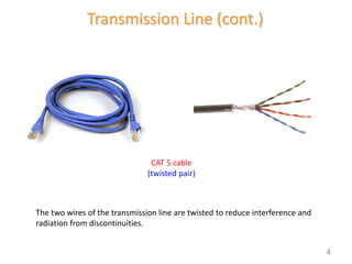
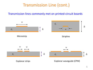
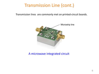
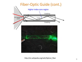
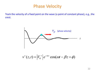
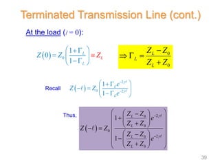
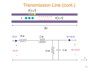
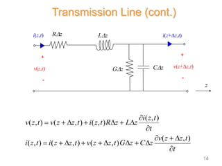
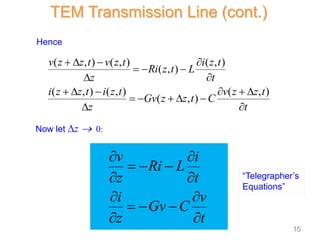
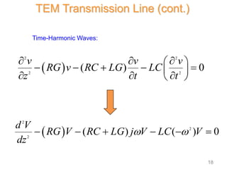
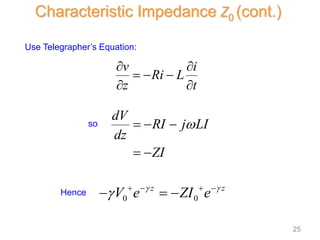
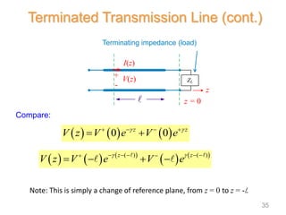
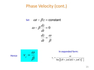
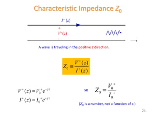
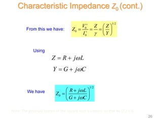
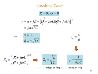
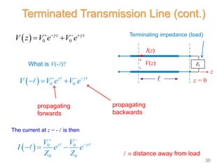
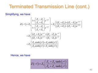
1) Transmission lines carry signals between two points by propagating waves along two parallel conductors. Common types include coaxial cable and printed circuit board traces. 2) Transmission lines are characterized by their per-unit-length inductance, capacitance, resistance, and conductance. The behavior of signals on the line is described by telegrapher's equations. 3) Waves on transmission lines travel at the phase velocity, defined as the ratio of frequency to phase constant. The characteristic impedance is determined by the line's inductance and capacitance.

1. KAVOSHCOM
RF Communication Circuits
Lecture 1: Transmission Lines

2. A wave guiding structure is one that carries a signal
(or power) from one point to another.
There are three common types:
 Transmission lines
 Fiber-optic guides
 Waveguides
Waveguiding Structures
2

3. Transmission Line
 Has two conductors running parallel
 Can propagate a signal at any frequency (in theory)
 Becomes lossy at high frequency
 Can handle low or moderate amounts of power
 Does not have signal distortion, unless there is loss
 May or may not be immune to interference
 Does not have Ez or Hz components of the fields (TEMz)
Properties
Coaxial cable (coax)
Twin lead
(shown connected to a 4:1
impedance-transforming balun)
3

4. Transmission Line (cont.)
CAT 5 cable
(twisted pair)
The two wires of the transmission line are twisted to reduce interference and
radiation from discontinuities.
4

5. Transmission Line (cont.)
Microstrip
h
w
er
er
w
Stripline
h
Transmission lines commonly met on printed-circuit boards
Coplanar strips
h
er
w w
Coplanar waveguide (CPW)
h
er
w
5

6. Transmission Line (cont.)
Transmission lines are commonly met on printed-circuit boards.
A microwave integrated circuit
Microstrip line
6

7. Fiber-Optic Guide
Properties
 Uses a dielectric rod
 Can propagate a signal at any frequency (in theory)
 Can be made very low loss
 Has minimal signal distortion
 Very immune to interference
 Not suitable for high power
 Has both Ez and Hz components of the fields
7

8. Fiber-Optic Guide (cont.)
Two types of fiber-optic guides:
1) Single-mode fiber
2) Multi-mode fiber
Carries a single mode, as with the mode on a
transmission line or waveguide. Requires the fiber
diameter to be small relative to a wavelength.
Has a fiber diameter that is large relative to a
wavelength. It operates on the principle of total internal
reflection (critical angle effect).
8

9. Fiber-Optic Guide (cont.)
http://en.wikipedia.org/wiki/Optical_fiber
Higher index core region
9

10. Waveguides
 Has a single hollow metal pipe
 Can propagate a signal only at high frequency:  > c
 The width must be at least one-half of a wavelength
 Has signal distortion, even in the lossless case
 Immune to interference
 Can handle large amounts of power
 Has low loss (compared with a transmission line)
 Has either Ez or Hz component of the fields (TMz or TEz)
Properties
http://en.wikipedia.org/wiki/Waveguide_(electromagnetism) 10

11.  Lumped circuits: resistors, capacitors,
inductors
neglect time delays (phase)
account for propagation and
time delays (phase change)
Transmission-Line Theory
 Distributed circuit elements: transmission lines
We need transmission-line theory whenever the length of
a line is significant compared with a wavelength.
11

12. Transmission Line
2 conductors
4 per-unit-length parameters:
C = capacitance/length [F/m]
L = inductance/length [H/m]
R = resistance/length [/m]
G = conductance/length [ /m or S/m]

Dz
12

13. Transmission Line (cont.)
z
D
 
,
i z t
+ + + + + + +
- - - - - - - - - -
 
,
v z t
x x x
B
13
RDz LDz
GDz CDz
z
v(z+Dz,t)
+
-
v(z,t)
+
-
i(z,t) i(z+Dz,t)

14. ( , )
( , ) ( , ) ( , )
( , )
( , ) ( , ) ( , )
i z t
v z t v z z t i z t R z L z
t
v z z t
i z t i z z t v z z t G z C z
t

  D  D  D

  D
  D   D D  D

Transmission Line (cont.)
14
RDz LDz
GDz CDz
z
v(z+Dz,t)
+
-
v(z,t)
+
-
i(z,t) i(z+Dz,t)

15. Hence
( , ) ( , ) ( , )
( , )
( , ) ( , ) ( , )
( , )
v z z t v z t i z t
Ri z t L
z t
i z z t i z t v z z t
Gv z z t C
z t
 D  
  
D 
 D    D
   D 
D 
Now let Dz  0:
v i
Ri L
z t
i v
Gv C
z t
 
  
 
 
  
 
“Telegrapher’s
Equations”
TEM Transmission Line (cont.)
15

16. To combine these, take the derivative of the first one with
respect to z:
2
2
2
2
v i i
R L
z z z t
i i
R L
z t z
v
R Gv C
t
v v
L G C
t t
   
 
    
   
 
  
 
    
  
 

 
   
 

 
 
 
  
 
 
 
Switch the
order of the
derivatives.
TEM Transmission Line (cont.)
16

17.  
2 2
2 2
( ) 0
v v v
RG v RC LG LC
z t t
  
 
    
 
  
 
The same equation also holds for i.
Hence, we have:
2 2
2 2
v v v v
R Gv C L G C
z t t t
   
   
      
   
   
   
TEM Transmission Line (cont.)
17

18.  
2
2
2
( ) ( ) 0
d V
RG V RC LG j V LC V
dz
 
     
 
2 2
2 2
( ) 0
v v v
RG v RC LG LC
z t t
  
 
    
 
  
 
TEM Transmission Line (cont.)
Time-Harmonic Waves:
18

19. Note that
= series impedance/length
   
2
2
2
( )
d V
RG V j RC LG V LC V
dz
 
   
2
( ) ( )( )
RG j RC LG LC R j L G j C
   
     
Z R j L
Y G j C


 
  = parallel admittance/length
Then we can write:
2
2
( )
d V
ZY V
dz

TEM Transmission Line (cont.)
19

20. Let
Convention:
Solution:
2
  ZY
( ) z z
V z Ae Be
 
 
 
 
1/2
( )( )
R j L G j C
  
  
 principal square root
2
2
2
( )
d V
V
dz


Then
TEM Transmission Line (cont.)
 is called the "propagation constant."
/2
j
z z e 

  
  
j
  
 
0, 0
 
 




attenuationcontant
phaseconstant
20

21. TEM Transmission Line (cont.)
0 0
( ) z z j z
V z V e V e e
  
     
 
Forward travelling wave (a wave traveling in the positive z direction):
 
 
 
 
 
0
0
0
( , ) Re
Re
cos
z j z j t
j z j z j t
z
v z t V e e e
V e e e e
V e t z
  
   

  
   
  
 


  
g

0
t 
z
0
z
V e 
 
2
g




2
g
 

The wave “repeats” when:
Hence:
21

22. Phase Velocity
Track the velocity of a fixed point on the wave (a point of constant phase), e.g., the
crest.
0
( , ) cos( )
z
v z t V e t z

  
  
  
z
vp (phase velocity)
22

23. Phase Velocity (cont.)
0
constant
 
 


 
 

t z
dz
dt
dz
dt
Set
Hence p
v



 
 
1/2
Im ( )( )
p
v
R j L G j C

 

 
In expanded form:
23

24. Characteristic Impedance Z0
0
( )
( )
V z
Z
I z



0
0
( )
( )
z
z
V z V e
I z I e


  
  


so 0
0
0
V
Z
I



+
V+(z)
-
I+ (z)
z
A wave is traveling in the positive z direction.
(Z0 is a number, not a function of z.)
24

25. Use Telegrapher’s Equation:
v i
Ri L
z t
 
  
 
so
dV
RI j LI
dz
ZI

  
 
Hence
0 0
z z
V e ZI e
 
    
  
Characteristic Impedance Z0 (cont.)
25

26. From this we have:
Using
We have
1/2
0
0
0
V Z Z
Z
I Y



 
    
 
Y G j C

 
1/2
0
R j L
Z
G j C


 

  

 
Characteristic Impedance Z0 (cont.)
Z R j L

 
Note: The principal branch of the square root is chosen, so that Re (Z0) > 0.
26

27.  
0
0
0 0
j z j j z
z z
z j z
V e e
V z V e V
V e e e
e
e
 
 

  


  

   


 
 
   
 
 
 
0
0 cos
c
, R
os
e j t
z
z
V e t
v z t V z
z
V z
e
e t



 
  

 
 









Note:
wave in +z
direction
wave in -z
direction
General Case (Waves in Both Directions)
27

28. Backward-Traveling Wave
0
( )
( )
V z
Z
I z



 0
( )
( )
V z
Z
I z


 
so
+
V -(z)
-
I - (z)
z
A wave is traveling in the negative z direction.
Note: The reference directions for voltage and current are the same as
for the forward wave.
28

29. General Case
0 0
0 0
0
( )
1
( )
z z
z z
V z V e V e
I z V e V e
Z
 
 
   
   
 
 
 
 
A general superposition of forward and
backward traveling waves:
Most general case:
Note: The reference
directions for voltage
and current are the
same for forward and
backward waves.
29
+
V(z)
-
I(z)
z

30.  
 
  
1
2
1
2
0
0 0
0 0
0 0
z z
z z
V z V e V e
V V
I z e e
Z
j R j L G j C
R j L
Z
G j
Z
C
 
 
    


   
 
 

 
   
 
 
 

 






I(z)
V(z)
+
-
z
 
2
m
g




[m/s]
p
v



guided wavelength  g
phase velocity  vp
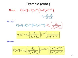
Summary of Basic TL formulas
30

31. Lossless Case
0, 0
R G
 
 
1/ 2
( )( )
j R j L G j C
j LC
    

    

so 0
LC

 


1/2
0
R j L
Z
G j C


 

  

 
0
L
Z
C

1
p
v
LC

p
v



(indep. of freq.)
(real and indep. of freq.)
31

32. Lossless Case (cont.)
1
p
v
LC

In the medium between the two conductors is homogeneous (uniform)
and is characterized by (e, ), then we have that
LC e

The speed of light in a dielectric medium is
1
d
c
e

Hence, we have that p d
v c

The phase velocity does not depend on the frequency, and it is always the
speed of light (in the material).
(proof given later)
32

33.   0 0
z z
V z V e V e
 
   
 
Where do we assign z = 0?
The usual choice is at the load.
I(z)
V(z)
+
-
z
ZL
z = 0
Terminating impedance (load)
Ampl. of voltage wave
propagating in negative z
direction at z = 0.
Ampl. of voltage wave
propagating in positive z
direction at z = 0.
Terminated Transmission Line
Note: The length l measures distance from the load: z
 
33

34. What if we know
@
V V z
 
 
and
   
0 0
V V V e 
   
  
     
   
z z
V z V e V e
 
  
 
   
   
0
V V e 
  
 
   
0 0
V V V e
  
   
Terminated Transmission Line (cont.)
  0 0
z z
V z V e V e
 
   
 
Hence
Can we use z = - l as
a reference plane?
I(z)
V(z)
+
-
z
ZL
z = 0
Terminating impedance (load)
34

35.      
   
( ) ( )
z z
V z V e V e
 
    
 
   
Terminated Transmission Line (cont.)
     
0 0
z z
V z V e V e
 
   
 
Compare:
Note: This is simply a change of reference plane, from z = 0 to z = -l.
I(z)
V(z)
+
-
z
ZL
z = 0
Terminating impedance (load)
35

36.   0 0
z z
V z V e V e
 
   
 
What is V(-l )?
  0 0
V V e V e
 
  
  
  0 0
0 0
V V
I e e
Z Z
 
 

  
propagating
forwards
propagating
backwards
Terminated Transmission Line (cont.)
l  distance away from load
The current at z = - l is then
I(z)
V(z)
+
-
z
ZL
z = 0
Terminating impedance (load)
36

37.    
2
0
0
1 L
V
I e e
Z
 


  
  2
0
0
0
0 0 1
V
V e
V V e e
e
V
V  
 


 
 

 
 
 

 
 
Total volt. at distance l
from the load
Ampl. of volt. wave prop.
towards load, at the load
position (z = 0).
Similarly,
Ampl. of volt. wave prop.
away from load, at the
load position (z = 0).
 
0
2
1 L
V e e
 
 
 
L  Load reflection coefficient
Terminated Transmission Line (cont.)
I(-l )
V(-l )
+
l
ZL
-
0,
Z 
l  Reflection coefficient at z = - l
37

38.    
   
 
 
 
2
0
2
2
0
0
2
0
1
1
1
1
L
L
L
L
V V e e
V
I e e
Z
V e
Z Z
I e
 
 


 




   
  
 
    
 
  

 
Input impedance seen “looking” towards load
at z = -l .
Terminated Transmission Line (cont.)
I(-l )
V(-l )
+
l
ZL
-
0,
Z 
 
Z 
38

39. At the load (l = 0):
  0
1
0
1
L
L
L
Z Z Z
 

  


 
Thus,
 
2
0
0
0
2
0
0
1
1
L
L
L
L
Z Z
e
Z Z
Z Z
Z Z
e
Z Z




 
 


 
 

 
 
 
 
 


 
 
 

 
 
Terminated Transmission Line (cont.)
0
0
L
L
L
Z Z
Z Z

  

 
2
0 2
1
1
L
L
e
Z Z
e




 
 
   

 
Recall
39

40. Simplifying, we have
 
 
 
0
0
0
tanh
tanh
L
L
Z Z
Z Z
Z Z


 

   
 

 
Terminated Transmission Line (cont.)
 
   
   
   
   
   
   
2
0
2
0 0 0
0 0 2
2 0 0
0
0
0 0
0
0 0
0
0
0
1
1
cosh sinh
cosh sinh
L
L L L
L L
L
L
L L
L L
L
L
Z Z
e
Z Z Z Z Z Z e
Z Z Z
Z Z Z Z e
Z Z
e
Z Z
Z Z e Z Z e
Z
Z Z e Z Z e
Z Z
Z
Z Z




 
 
 
 




 
 
 
 


 
   
   
 
 
    
 
    
 
  

 
 
 

 
 
 
  
  
 
  
 
 

 
 




Hence, we have
40

41.    
   
 
2
0
2
0
0
2
0 2
1
1
1
1
j j
L
j j
L
j
L
j
L
V V e e
V
I e e
Z
e
Z Z
e
 
 


 




   
  
 
 
   

 
Impedance is periodic
with period g/2
2
/ 2
g
g
 






 
Terminated Lossless Transmission Line
j j
   
  
Note:      
tanh tanh tan
j j
  
 
tan repeats when
 
 
 
0
0
0
tan
tan
L
L
Z jZ
Z Z
Z jZ


 

   
 

 
41

42. For the remainder of our transmission line discussion we will assume that the
transmission line is lossless.
   
   
 
 
 
 
 
2
0
2
0
0
2
0 2
0
0
0
1
1
1
1
tan
tan
j j
L
j j
L
j
L
j
L
L
L
V V e e
V
I e e
Z
V e
Z Z
I e
Z jZ
Z
Z jZ
 
 




 




   
  
  
 
    
 
 
 

  
 

 
0
0
2
L
L
L
g
p
Z Z
Z Z
v






 



Terminated Lossless Transmission Line
I(-l )
V(-l )
+
l
ZL
-
0 ,
Z 
 
Z 
42

43. Matched load: (ZL=Z0)
0
0
0
L
L
L
Z Z
Z Z

  

For any l
No reflection from the load
A
Matched Load
I(-l )
V(-l )
+
l
ZL
-
0 ,
Z 
 
Z 
  0
Z Z
  
 
 
0
0
0
j
j
V V e
V
I e
Z


 


  
 
43

44. Short circuit load: (ZL = 0)
   
0
0
0
0
1
0
tan
L
Z
Z
Z jZ 

   

  
Always imaginary!
Note:
B
2
g
 


  sc
Z jX
  
S.C. can become an O.C.
with a g/4 trans. line
0 1/4 1/2 3/4
g
/ 
XSC
inductive
capacitive
Short-Circuit Load
l
0 ,
Z 
 
0 tan
sc
X Z 

44

45. Using Transmission Lines to Synthesize Loads
A microwave filter constructed from microstrip.
This is very useful is microwave engineering.
45

46.  
 
 
0
0
0
tan
tan
L
in
L
Z jZ d
Z Z d Z
Z jZ d


 

    
 

 
  in
TH
in TH
Z
V d V
Z Z
 
    

 
I(-l)
V(-l)
+
l
ZL
-
0
Z 

ZTH
VTH
d
Zin
+
-
ZTH
VTH
+
Zin
V(-d)
+
-
Example
Find the voltage at any point on the line.
46

47. Note:    
0
2
1 j
L
j
V V e e
 
 



0
0
L
L
L
Z Z
Z Z

 

   
2
0 1
j d j d in
TH
in TH
L
V d
Z
Z
e V
Z
V e  
 
  
 
  

 
   
2
2
1
1
j
j d
in L
TH j d
m TH L
Z e
V V e
Z Z e




 

   
 
     
  
 
 
At l = d:
Hence
Example (cont.)
0 2
1
1
j d
in
TH j d
in TH L
Z
V V e
Z Z e


 

   
     
 
 
 
47

48. Some algebra:  
2
0 2
1
1
j d
L
in j d
L
e
Z Z d Z
e




 

    

 
 
   
 
   
 
2
2
0 2
0
2 2
2
0
0 2
2
0
2
0 0
2
0
2
0 0
0
1
1
1
1 1
1
1
1
1
1
j d
L
j d
j d
L
L
j d j d
j d
L TH L
L
TH
j d
L
j d
L
j d
TH L TH
j d
L
j d
TH TH
L
TH
in
in TH
e
Z
Z e
e
Z e Z e
e
Z Z
e
Z e
Z Z e Z Z
e
Z
Z
Z
Z Z
Z Z Z
e
Z Z
Z



 









 






 
 
   
 
 
  
      
 

 
 
 
 

  


 
 
  
  

     

 

 
2
0
2
0 0
0
1
1
j d
L
j d
TH TH
L
TH
e
Z Z Z Z
e
Z Z




 
 
 
  

     

 
Example (cont.)
48

49.    
2
0
2
0
1
1
j
j d L
TH j d
TH S L
Z e
V V e
Z Z e




 

   

     
  
   
2
0
2
0
1
1
j d
in L
j d
in TH TH S L
Z Z e
Z Z Z Z e




  
 
   
   
  
where 0
0
TH
S
TH
Z Z
Z Z

 

Example (cont.)
Therefore, we have the following alternative form for the result:
Hence, we have
49

50.    
2
0
2
0
1
1
j
j d L
TH j d
TH S L
Z e
V V e
Z Z e




 

   

     
  
   
Example (cont.)
I(-l)
V(-l)
+
l
ZL
-
0
Z 

ZTH
VTH
d
Zin
+
-
Voltage wave that would exist if there were no reflections from
the load (a semi-infinite transmission line or a matched load).
50

51.  
 
       
2 2
2 2 2 2
0
0
1 j d j d
L L S
j d j d j d j d
TH L S L L S L S
TH
e e
Z
V d V e e e e
Z Z
 
   
 
   
 
    
 
  
   
          
     
 

 
 

 
Example (cont.)
ZL
0
Z 

ZTH
VTH
d
+
-
Wave-bounce method (illustrated for l = d):
51

52. Example (cont.)
 
   
   
2
2 2
2
2 2 2
0
0
1
1
j d j d
L S L S
j d j d j d
TH L L S L S
TH
e e
Z
V d V e e e
Z Z
 
  
 
  
 
      
 
  
 
          
  
 
 

  

 
 
Geometric series:
2
0
1
1 , 1
1
n
n
z z z z
z


     


 
 
       
2 2
2 2 2 2
0
0
1 j d j d
L L S
j d j d j d j d
TH L S L L S L S
TH
e e
Z
V d V e e e e
Z Z
 
   
 
   
 
    
 
  
   
          
     
 

 
 

 
2
j d
L S
z e 

  
52

53. Example (cont.)
or
 
2
0
2
0
2
1
1
1
1
j d
L s
TH
j d
TH
L j d
L s
e
Z
V d V
Z Z
e
e






 
 
 
  
    
 

   
 
 
 
 
 
 
 
2
0
2
0
1
1
j d
L
TH j d
TH L s
Z e
V d V
Z Z e




  

    
  
  
This agrees with the previous result (setting l = d).
Note: This is a very tedious method – not recommended.
Hence
53

54. 0
0
0
tan
tan
L T
in T
T L
Z jZ
Z Z
Z jZ


 

  

 
2
4 4 2
g g
g
 
 
 

  
0
0
T
in T
L
jZ
Z Z
jZ
 
   
 
0
2
0
0
0
in in
T
L
Z Z
Z
Z
Z
   
 
Quarter-Wave Transformer
2
0T
in
L
Z
Z
Z

so
 
1/2
0 0
T L
Z Z Z

Hence
This requires ZL to be real.
ZL
Z0 Z0T
Zin
54

55.   2
0 1 L
j j
L
V V e e
 
 
   
   
 
2
0
2
0
1
1 L
j j
L
j
j j
L
V V e e
V e e e
 

 
 
 
   
  
 
 
max 0
min 0
1
1
L
L
V V
V V


  
  
  max
min
V
V

VoltageStanding WaveRatio VSWR
Voltage Standing Wave Ratio
I(-l )
V(-l )
+
l
ZL
-
0 ,
Z 
1
1
L
L
 

 
VSWR
z
1+ L

1
1- L

0
( )
V z
V 
/ 2
z 
D 
0
z 
55