Downloaded 30 times
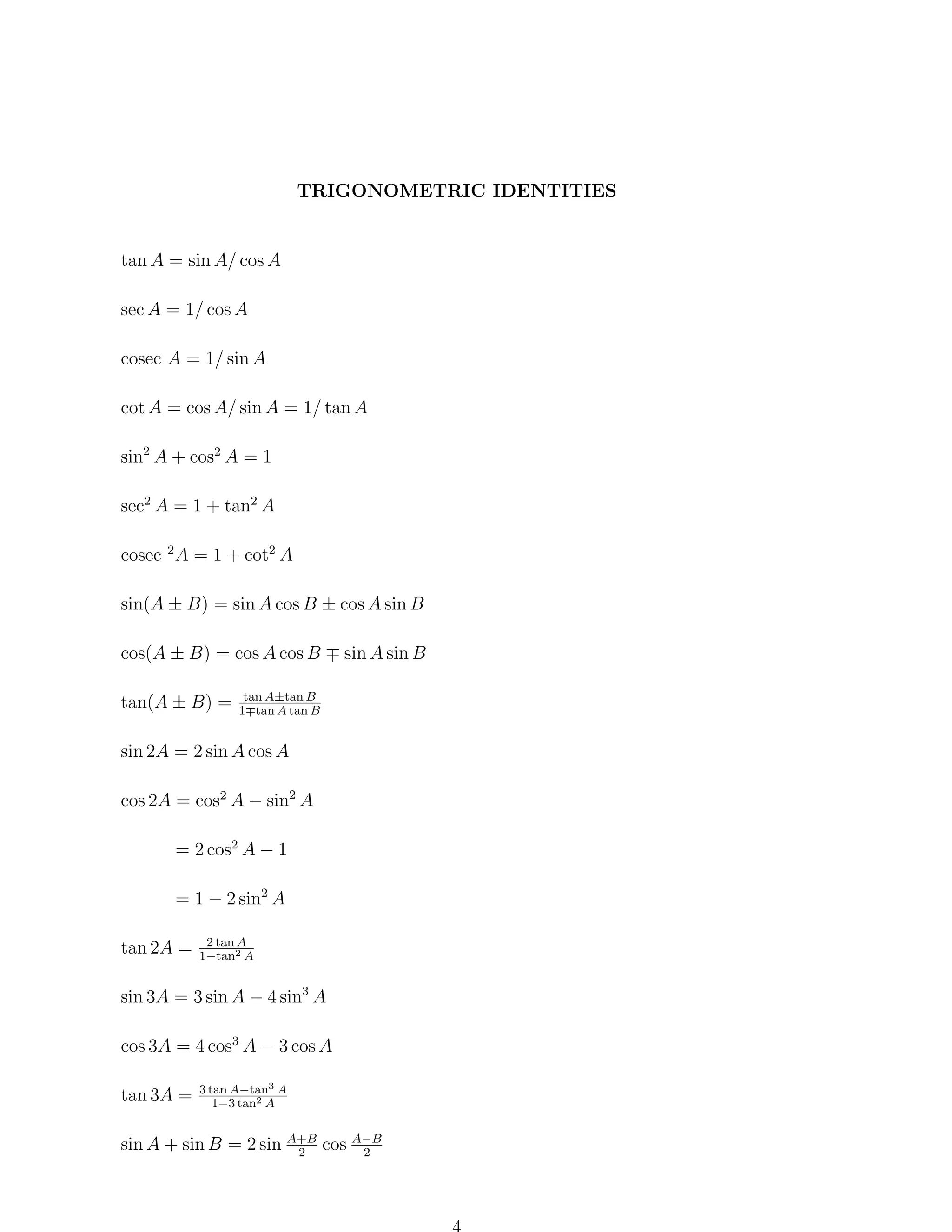
![COMPLEX NUMBERS
i=
√
−1
Note:- ‘j’ often used rather than ‘i’.
Exponential Notation
eiθ = cos θ + i sin θ
De Moivre’s theorem
[r(cos θ + i sin θ)]n = rn (cos nθ + i sin nθ)
nth roots of complex numbers
If z = reiθ = r(cos θ + i sin θ) then
z 1/n =
√ i(θ+2kπ)/n
n
re
,
k = 0, ±1, ±2, ...
HYPERBOLIC IDENTITIES
cosh x = (ex + e−x ) /2
tanh x = sinh x/ cosh x
sechx = 1/ cosh x
sinh x = (ex − e−x ) /2
cosechx = 1/ sinh x
coth x = cosh x/ sinh x = 1/ tanh x
cosh ix = cos x
sinh ix = i sin x
cos ix = cosh x
sin ix = i sinh x
cosh2 A − sinh2 A = 1
sech2 A = 1 − tanh2 A
cosech 2 A = coth2 A − 1](https://image.slidesharecdn.com/universityofmanchestermathematicalformulatables-140210113038-phpapp01/75/University-of-manchester-mathematical-formula-tables-6-2048.jpg)
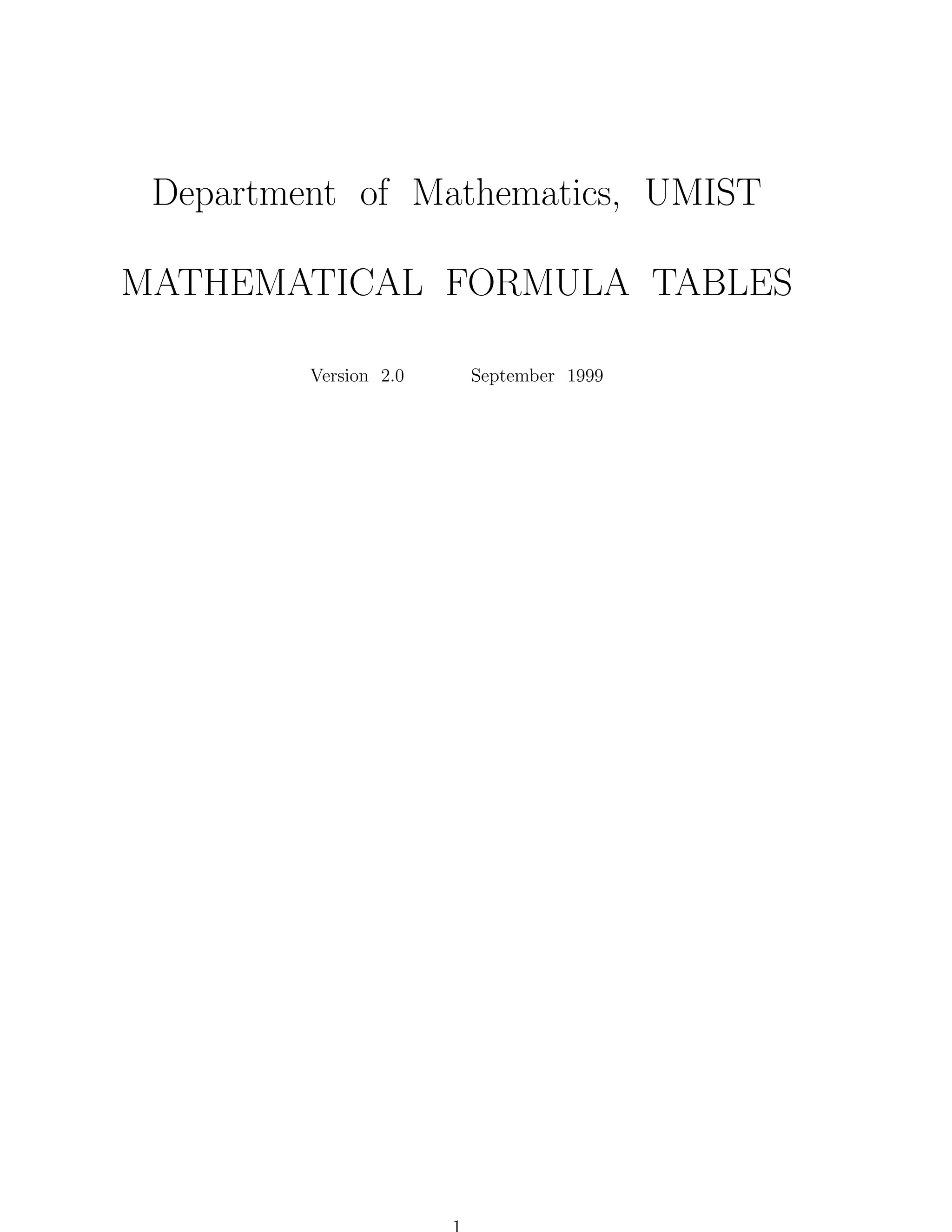
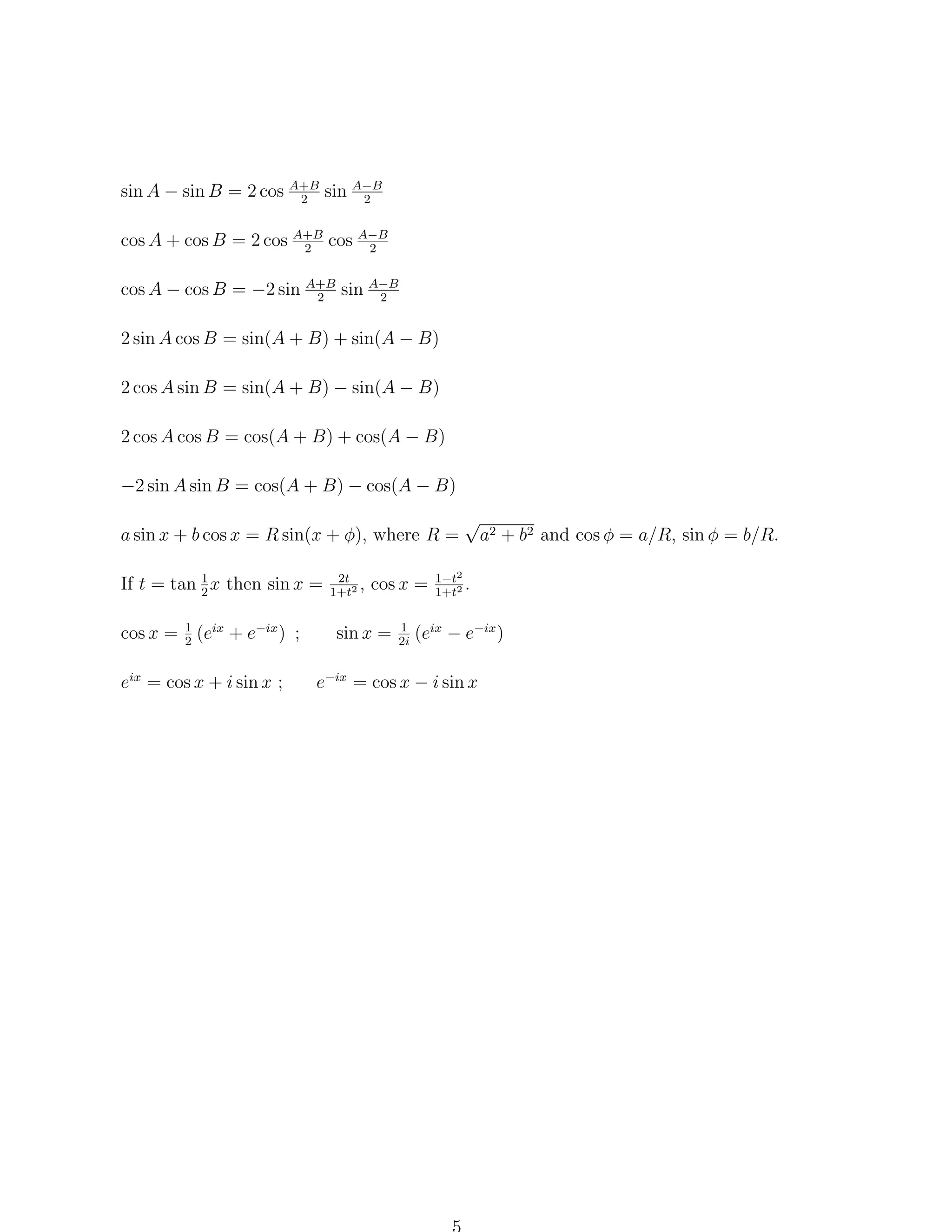
![Product Rule
d
dv
du
(u(x)v(x)) = u(x) + v(x)
dx
dx
dx
Quotient Rule
d
dx
u(x)
v(x)
=
dv
v(x) du − u(x) dx
dx
[v(x)]2
Chain Rule
d
(f (g(x))) = f (g(x)) × g (x)
dx
Leibnitz’s theorem
n(n − 1) (n−2) (2)
n!
dn
.g +...+
f (n−r) .g (r) +...+f.g (n)
(f.g) = f (n) .g+nf (n−1) .g (1) +
f
n
dx
2!
(n − r)!r!](https://image.slidesharecdn.com/universityofmanchestermathematicalformulatables-140210113038-phpapp01/75/University-of-manchester-mathematical-formula-tables-10-2048.jpg)

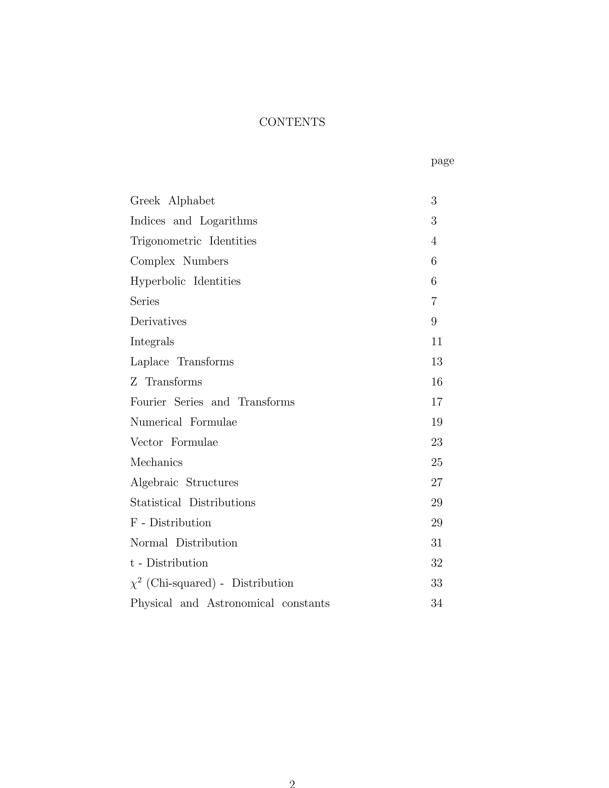
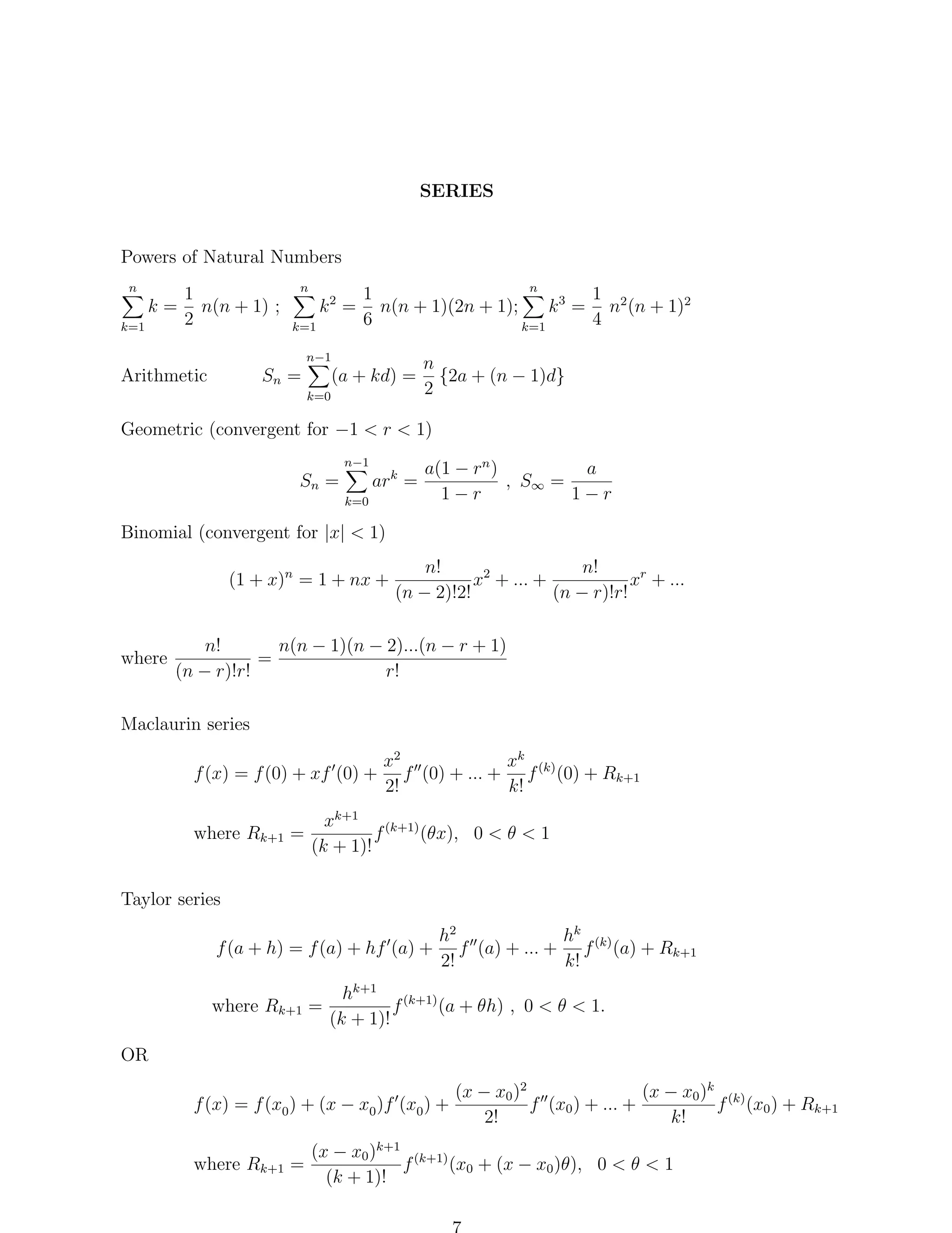
![Chebyshev Polynomials
Tn (x) = cos n(cos−1 x)
To (x) = 1
Un−1 (x) =
T1 (x) = x
Tn (x)
sin [n(cos−1 x)]
√
=
n
1 − x2
Tm (Tn (x)) = Tmn (x).
Tn+1 (x) = 2xTn (x) − Tn−1 (x)
Un+1 (x) = 2xUn (x) − Un−1 (x)
1 Tn+1 (x) Tn−1 (x)
Tn (x)dx =
−
+ constant,
2
n+1
n−1
where
and
1
f (x) = a0 T0 (x) + a1 T1 (x)...aj Tj (x) + ...
2
2 π
aj =
f (cos θ) cos jθdθ
π 0
f (x)dx = constant +A1 T1 (x) + A2 T2 (x) + ...Aj Tj (x) + ...
where Aj = (aj−1 − aj+1 )/2j
j≥1
n≥2
j≥0](https://image.slidesharecdn.com/universityofmanchestermathematicalformulatables-140210113038-phpapp01/75/University-of-manchester-mathematical-formula-tables-22-2048.jpg)
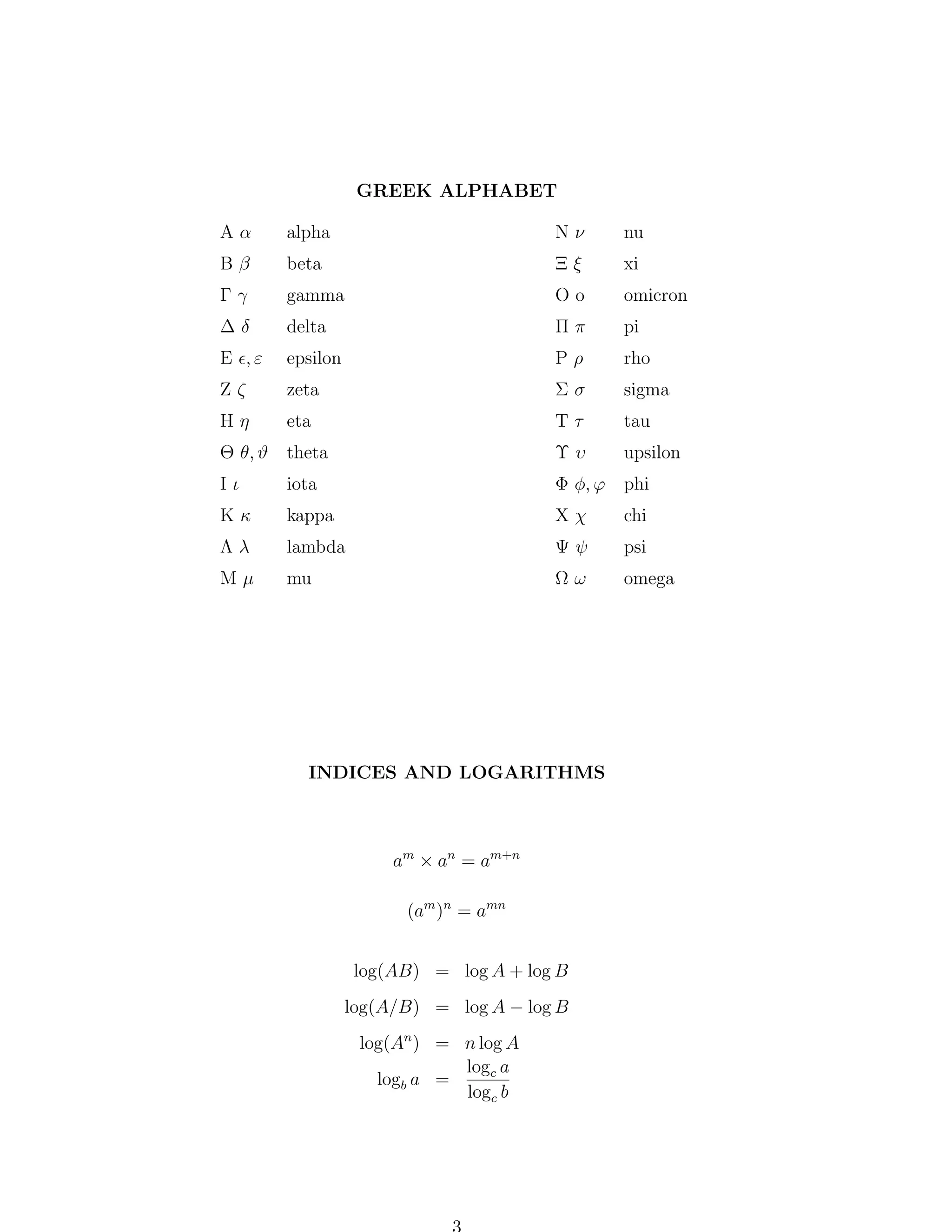
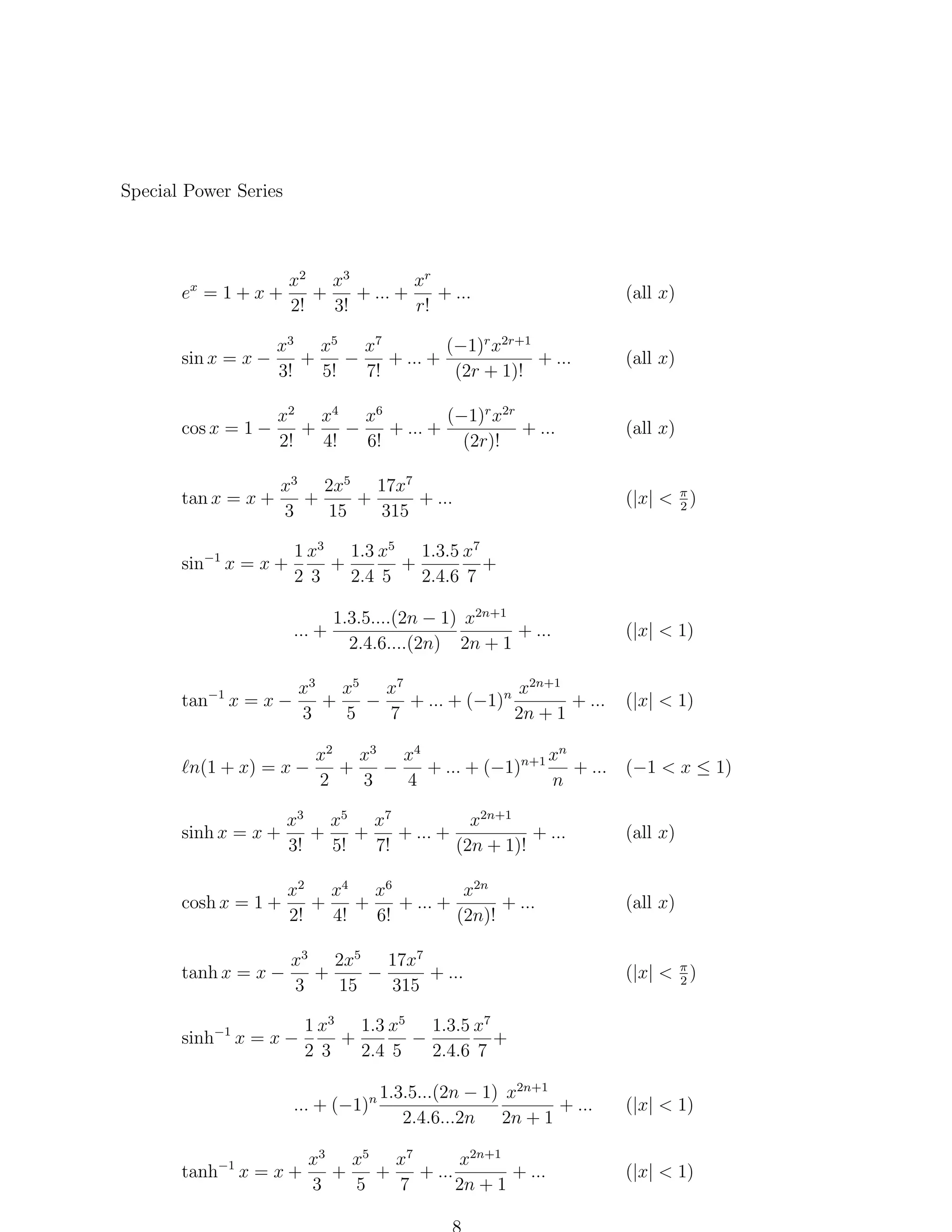
![VECTOR FORMULAE
Scalar product a.b = ab cos θ = a1 b1 + a2 b2 + a3 b3
i
j
k
n
Vector product a × b = ab sin θˆ = a1 a2 a3
b1 b2 b3
= (a2 b3 − a3 b2 )i + (a3 b1 − a1 b3 )j + (a1 b2 − a2 b1 )k
Triple products
a1 a2 a3
[a, b, c] = (a × b).c = a.(b × c) = b1 b2 b3
c1 c2 c3
a × (b × c) = (a.c)b − (a.b)c
Vector Calculus
≡
grad φ ≡
φ, div A ≡
div grad φ ≡
.(
2
.A, curl A ≡
φ) ≡
div curl A = 0
∂ ∂ ∂
, ,
∂x ∂y ∂z
2
×A
φ (for scalars only)
curl grad φ ≡ 0
A = grad div A − curl curl A
(αβ) = α
β+β
α
div (αA) = α div A + A.( α)
curl (αA) = α curl A − A × ( α)
div (A × B) = B. curl A − A. curl B
curl (A × B) = A div B − B div A + (B.
)A − (A.
)B](https://image.slidesharecdn.com/universityofmanchestermathematicalformulatables-140210113038-phpapp01/75/University-of-manchester-mathematical-formula-tables-23-2048.jpg)
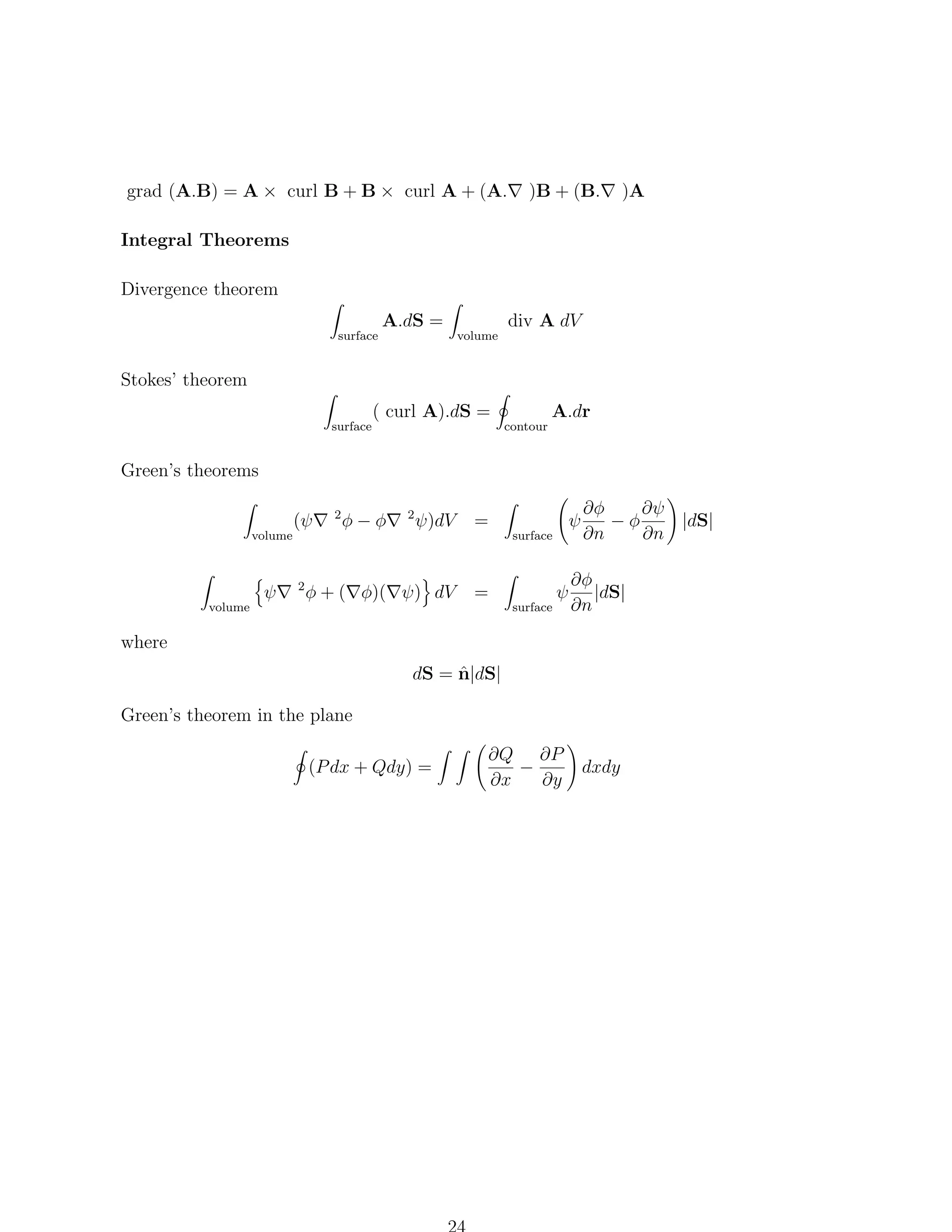
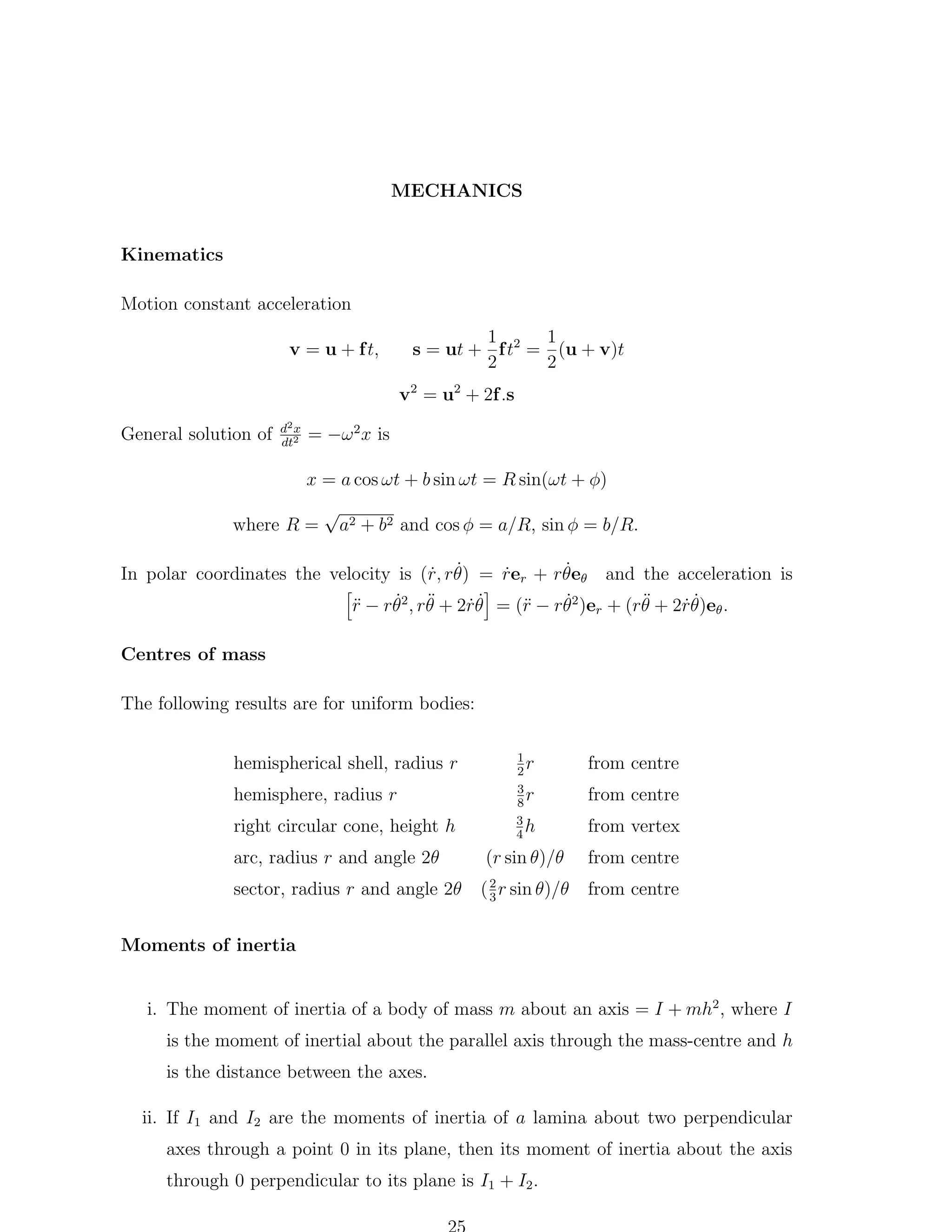
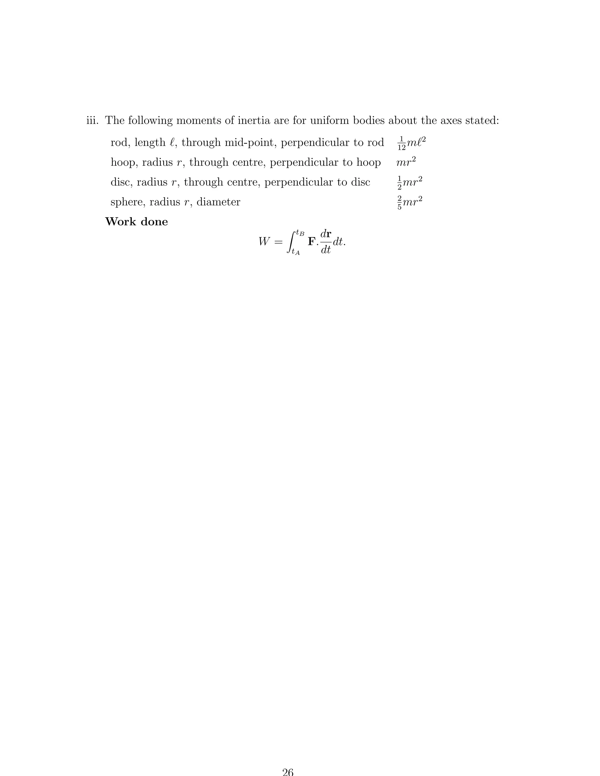
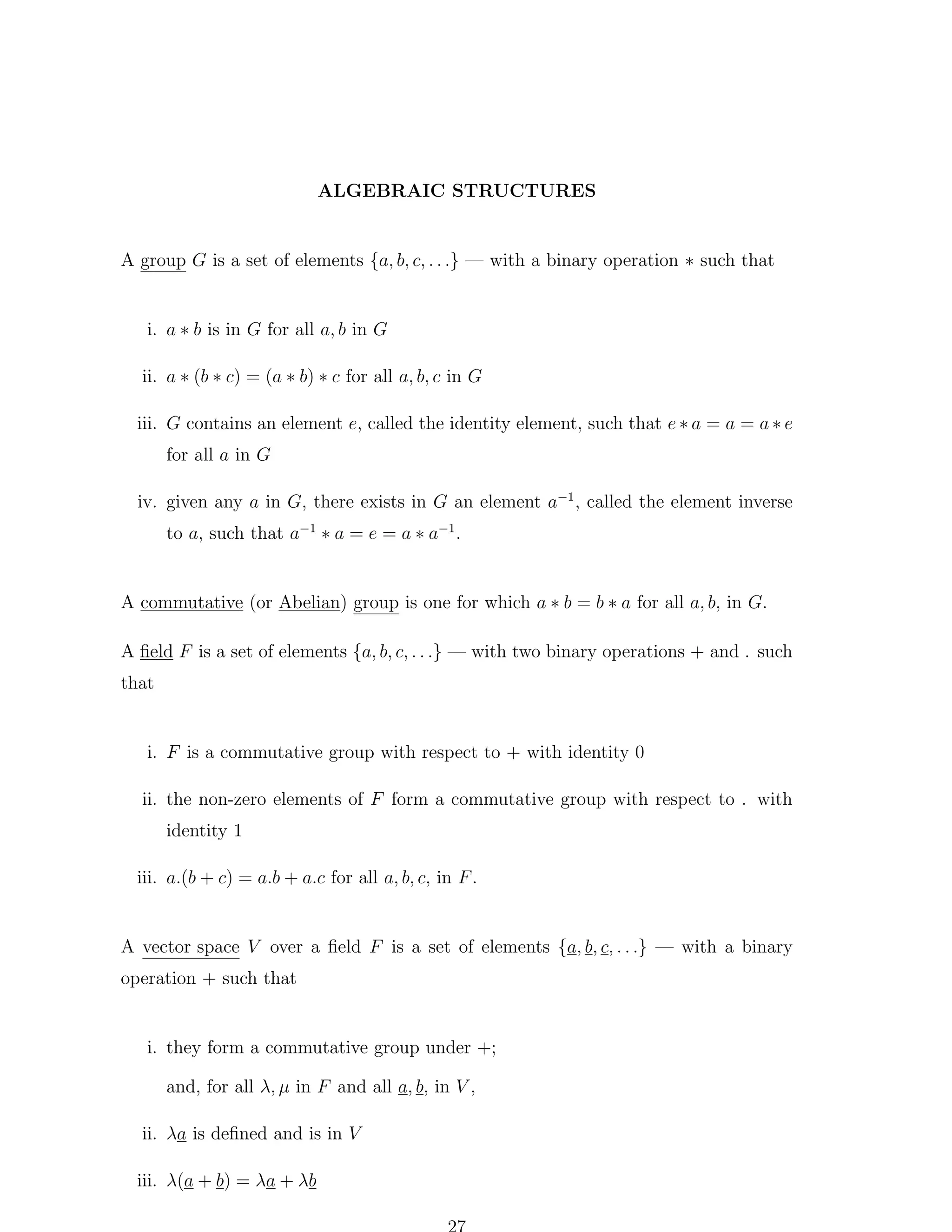
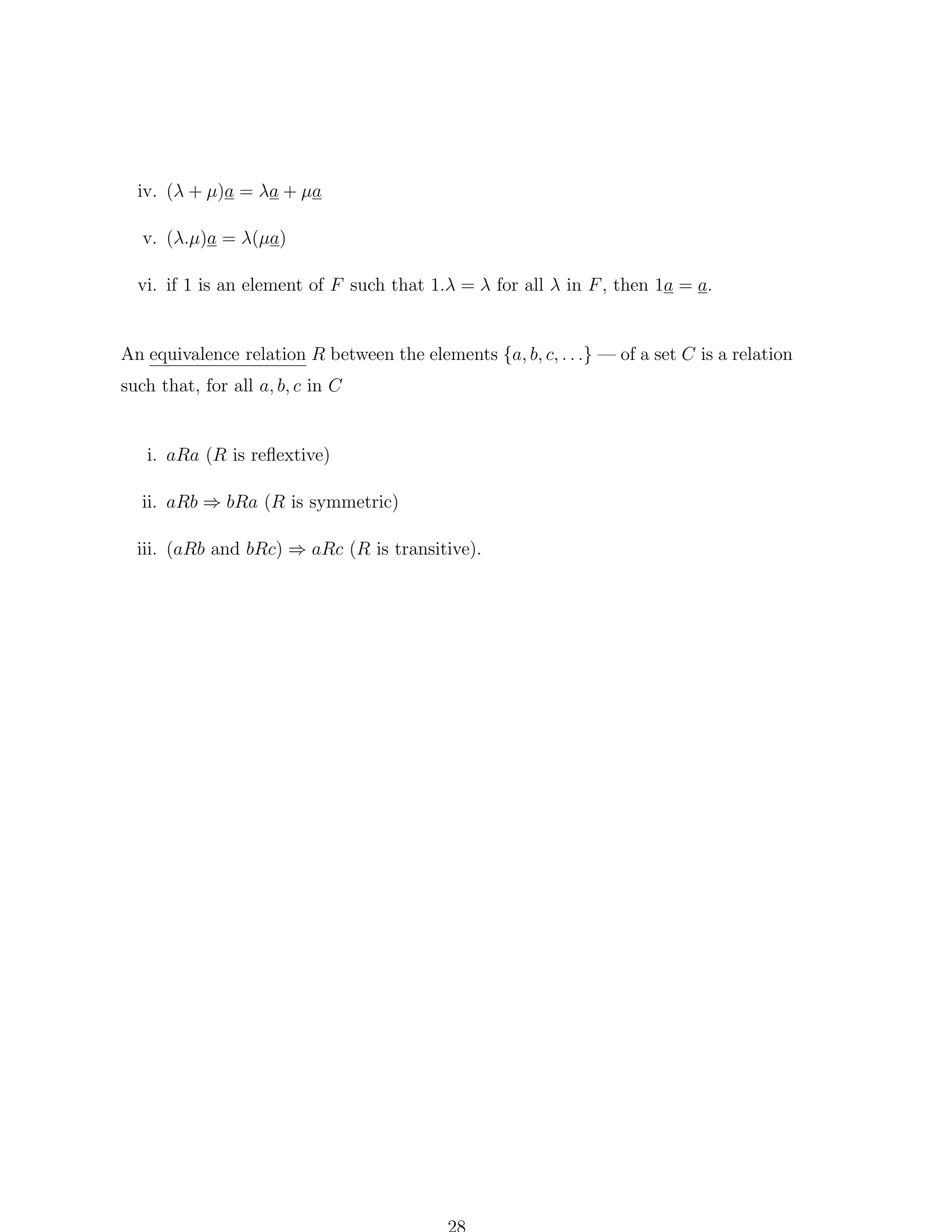
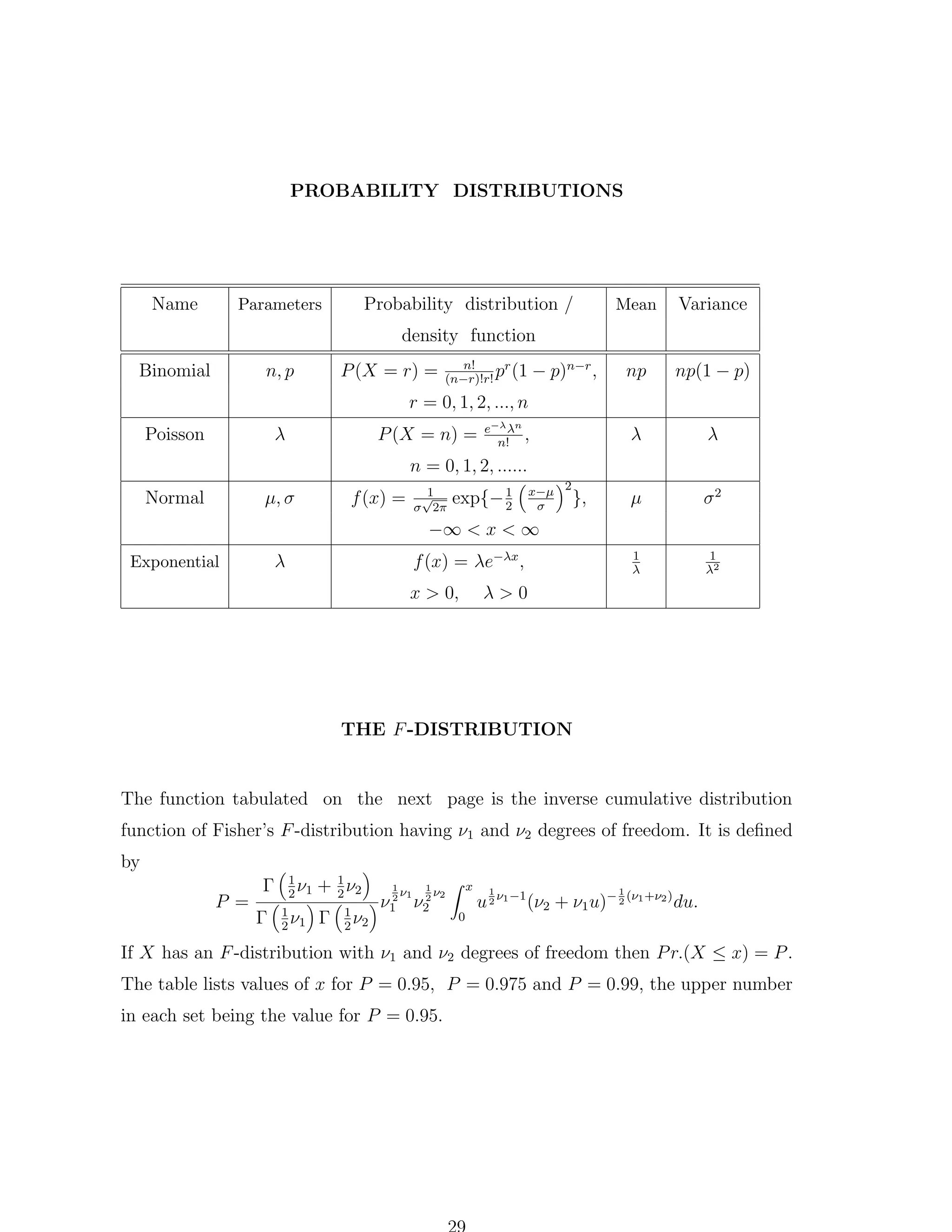
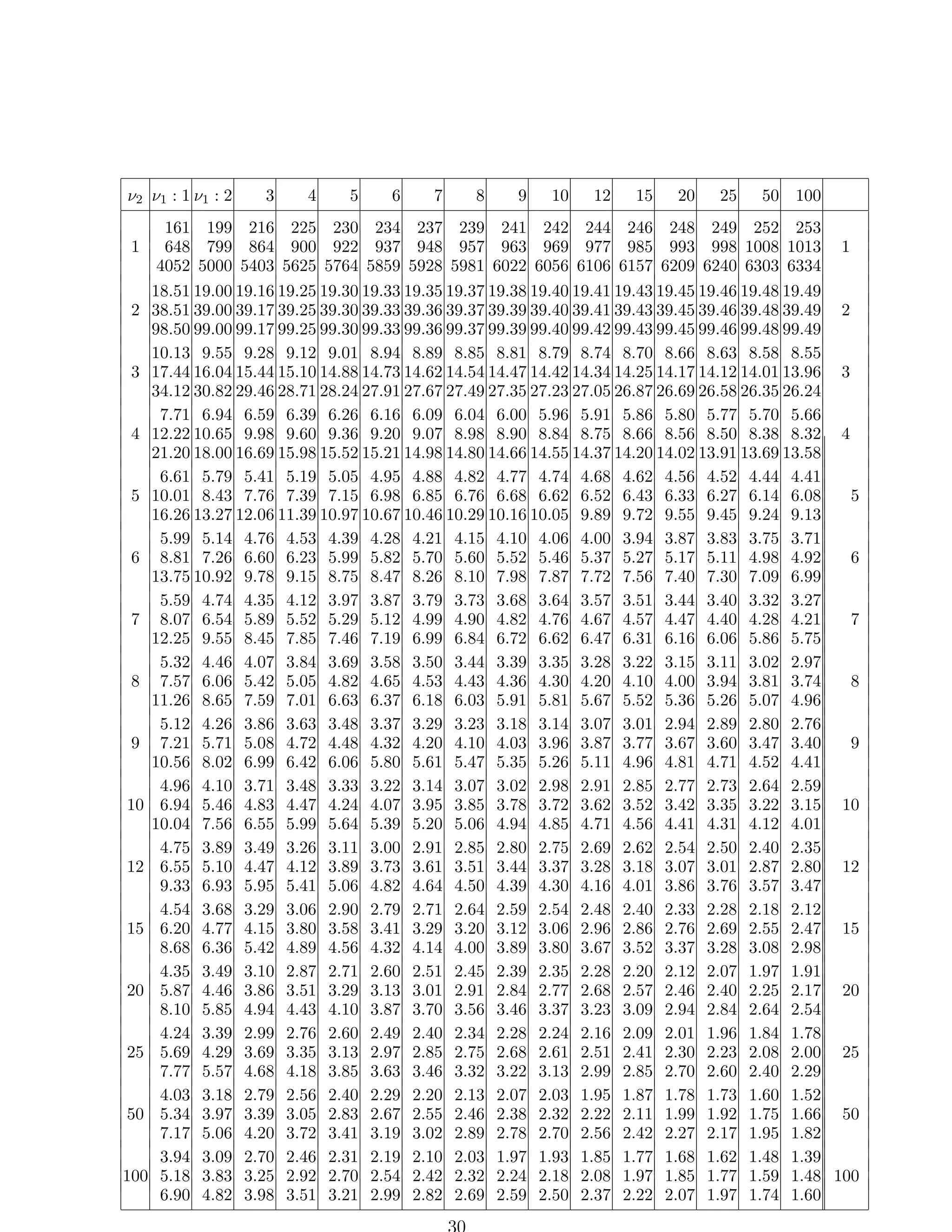
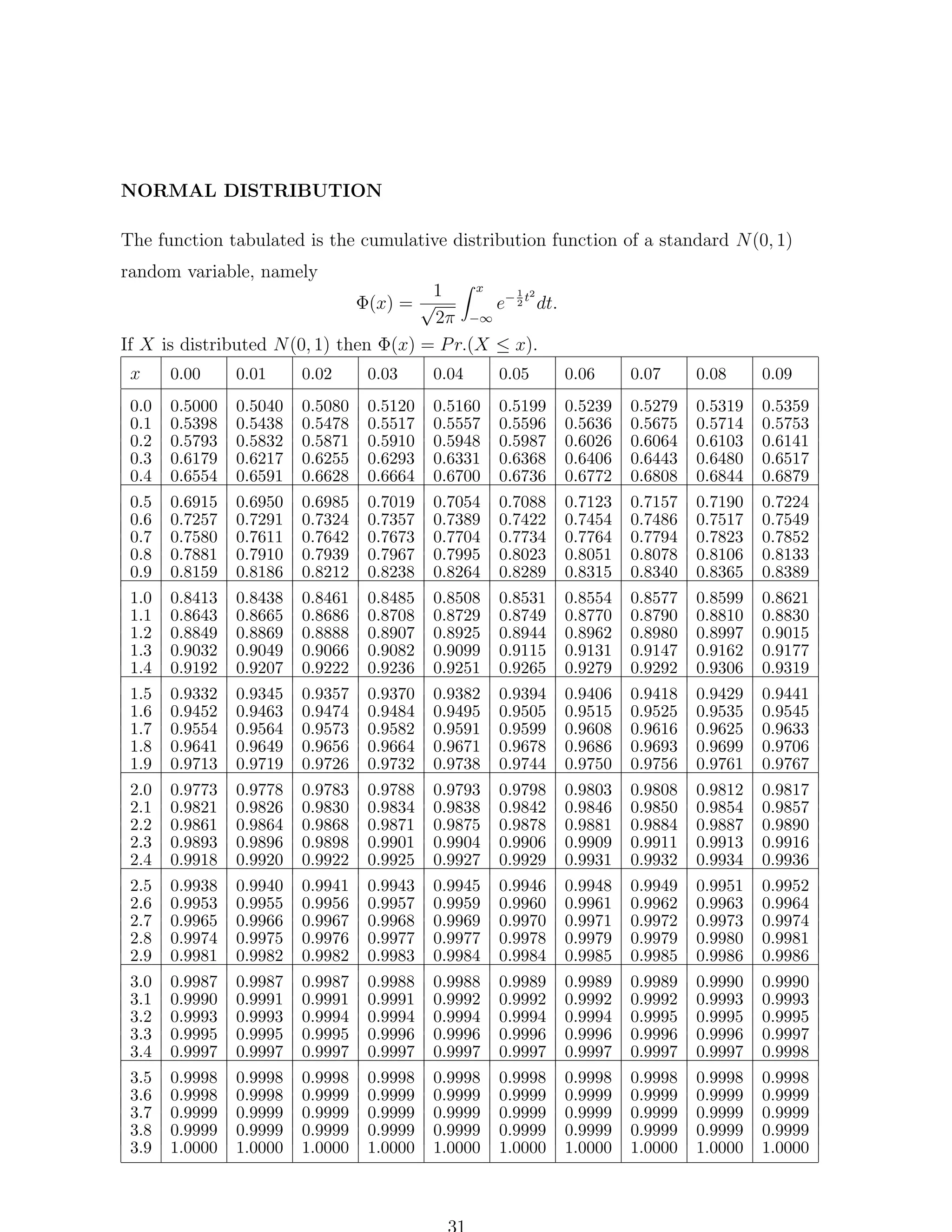
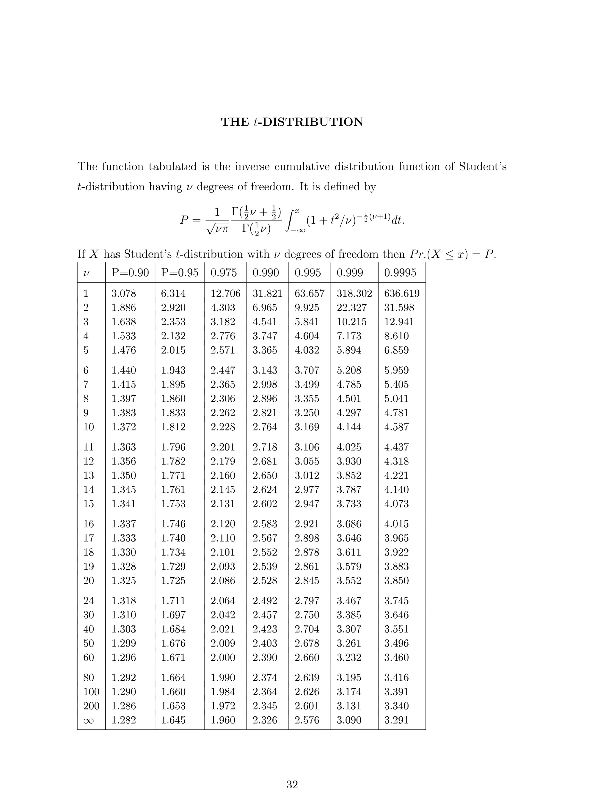
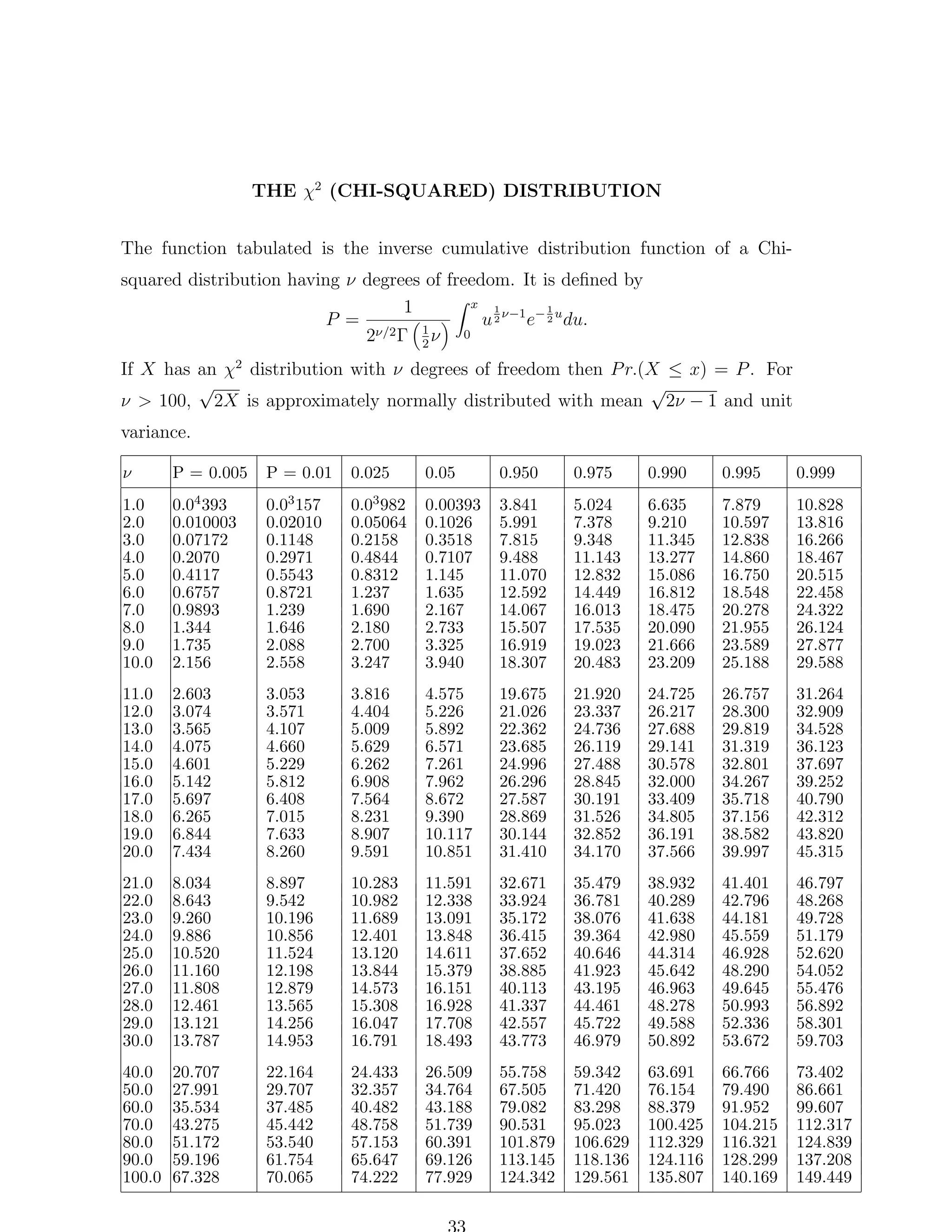
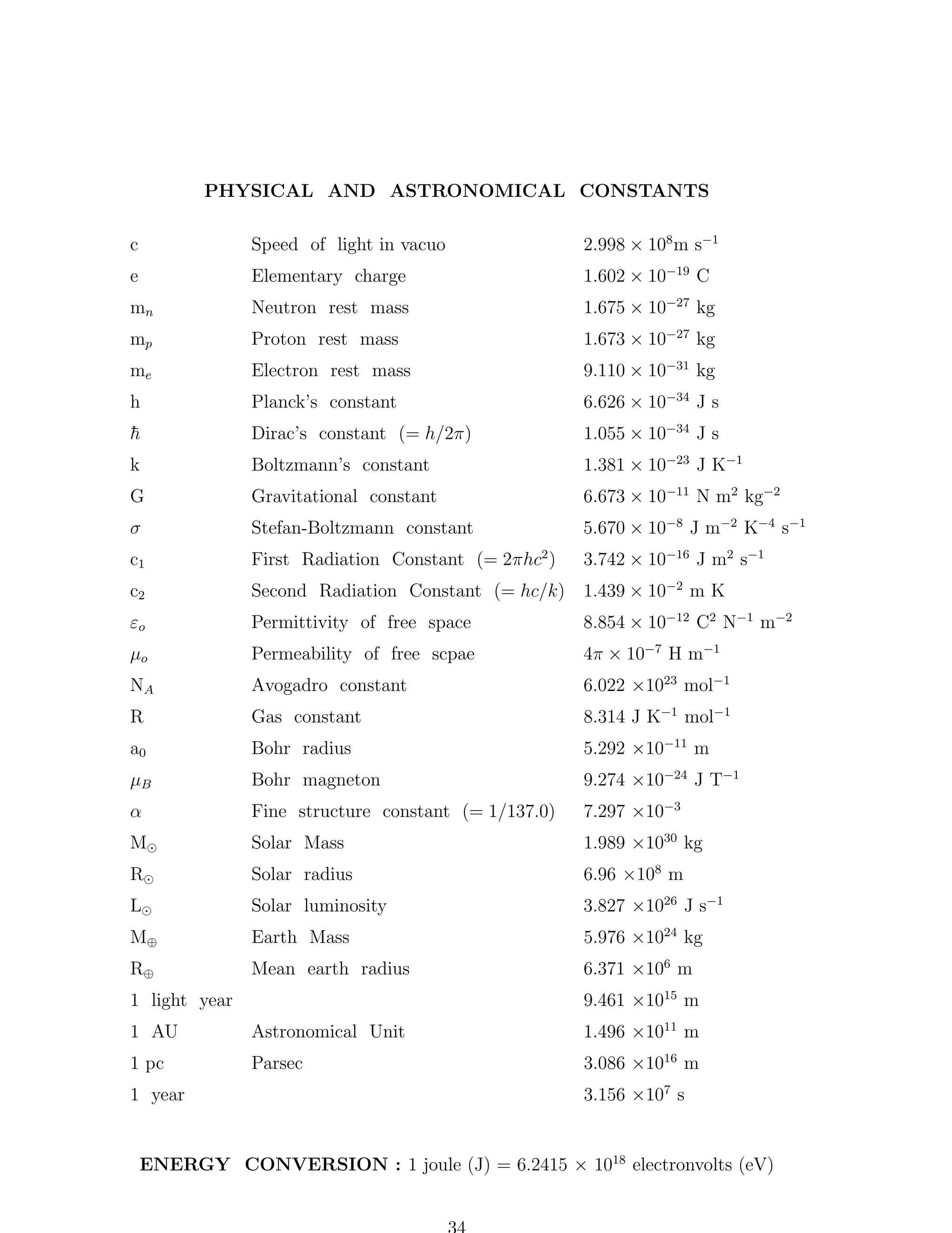

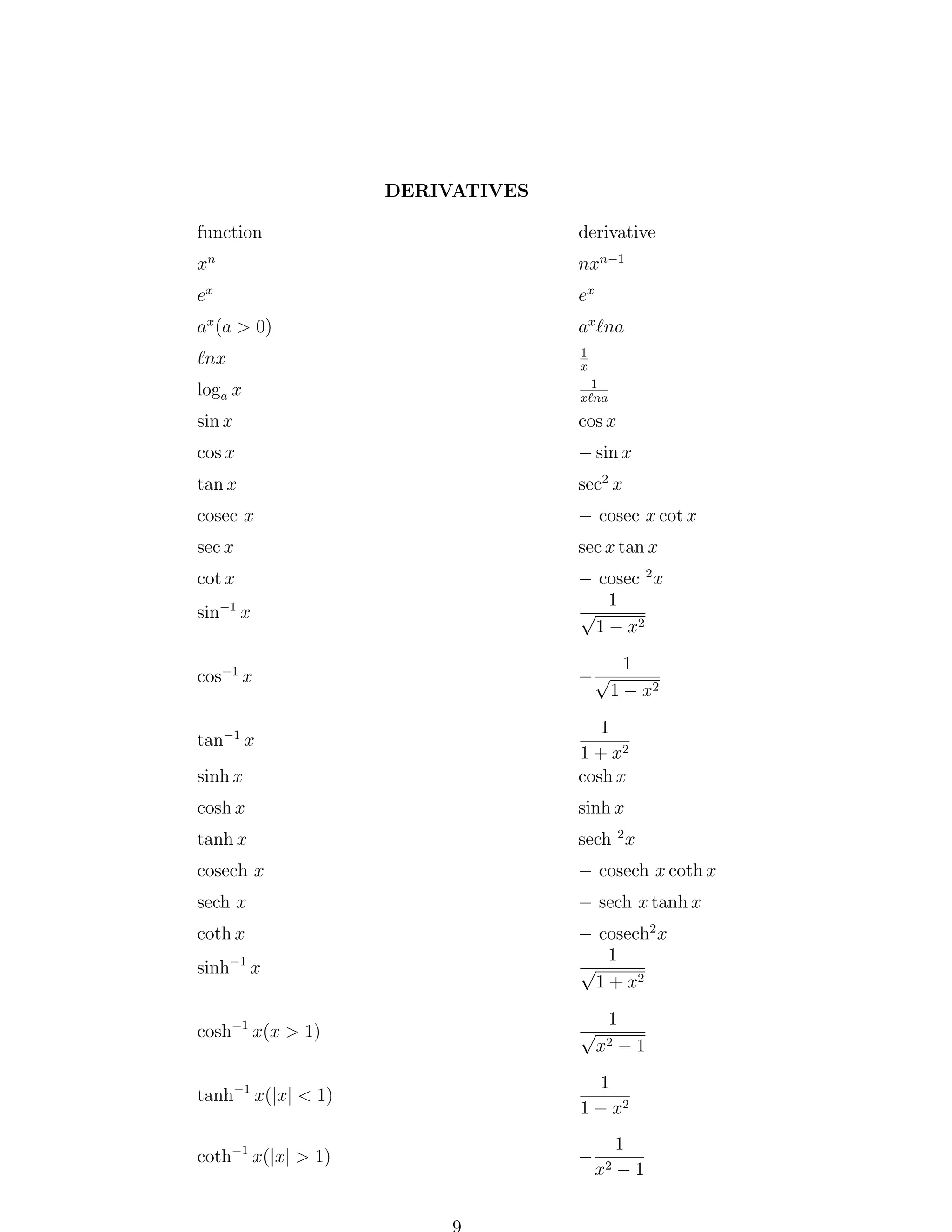
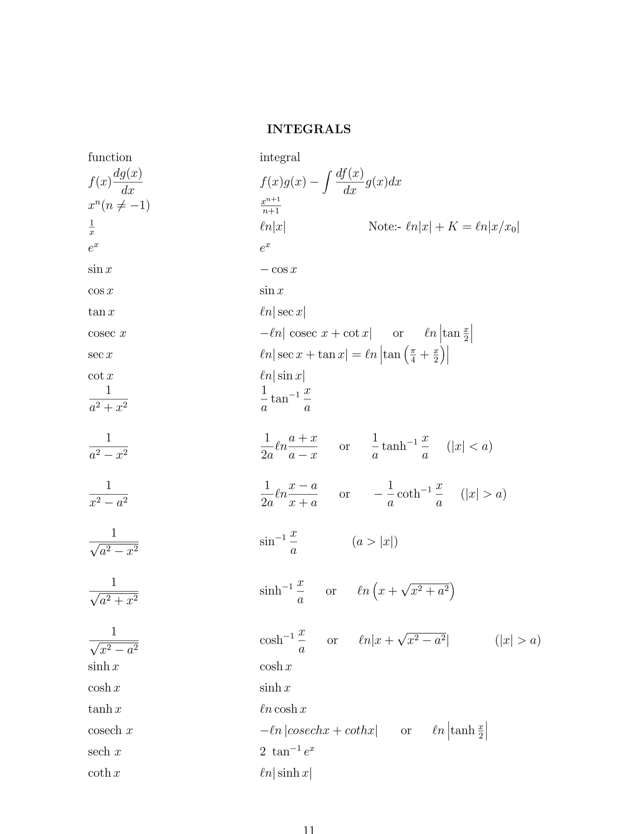
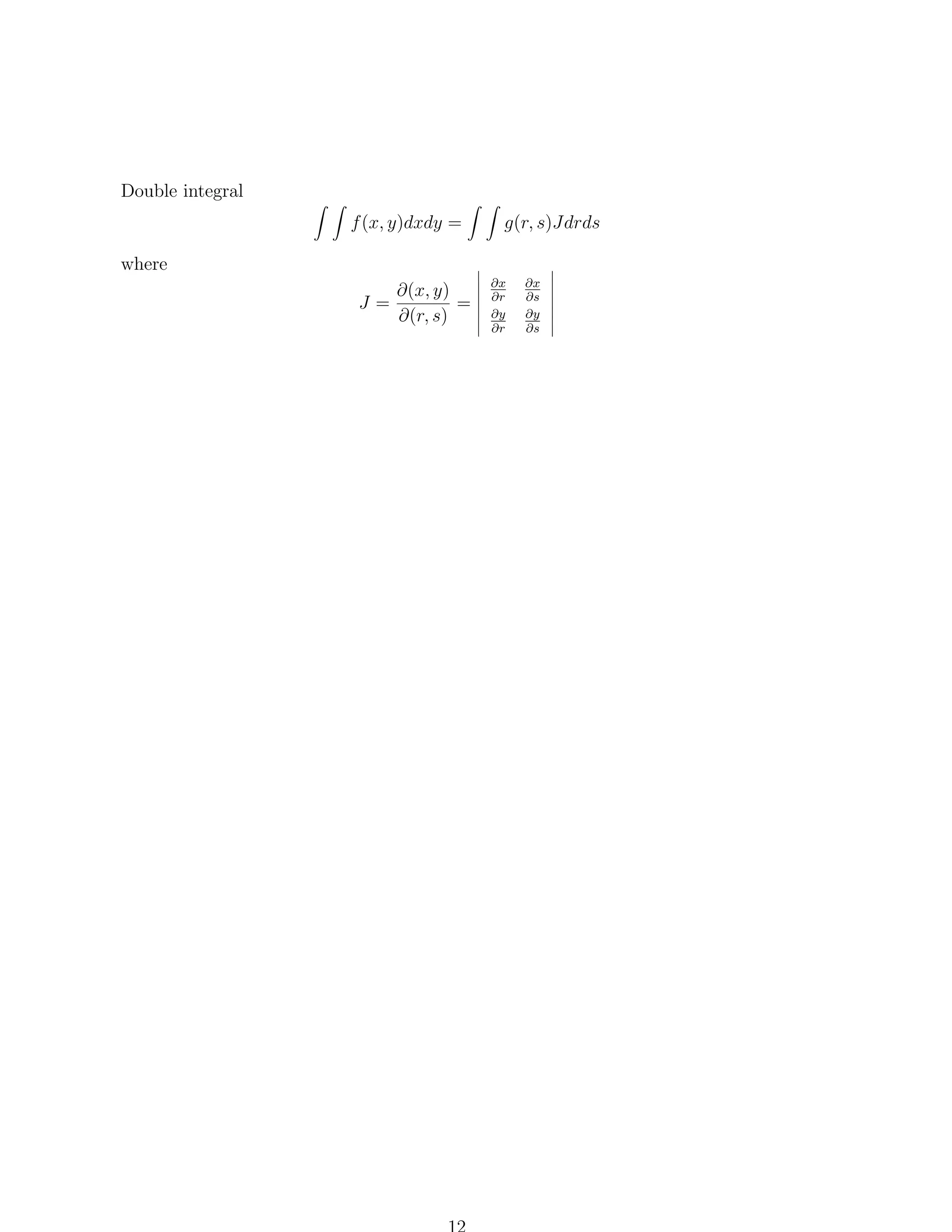
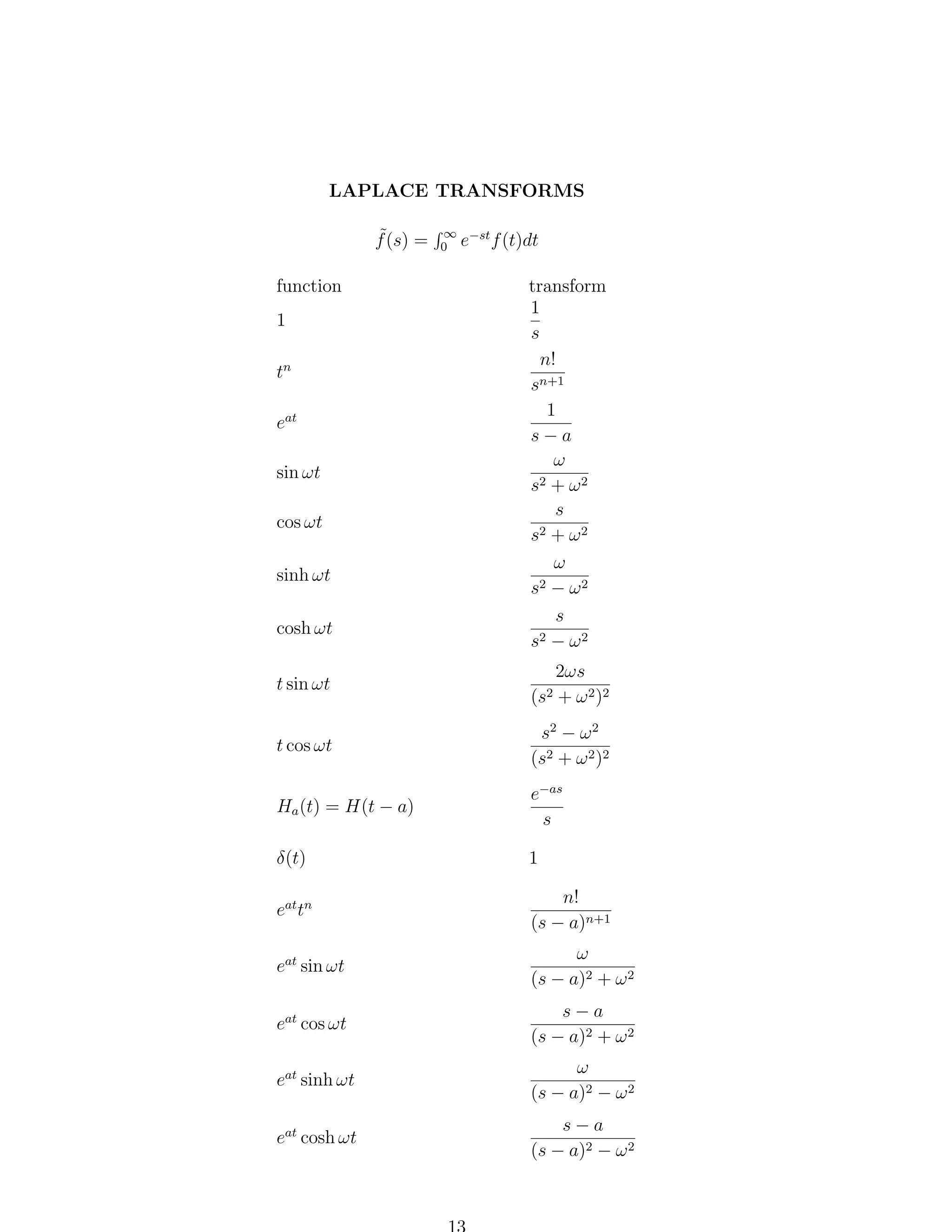
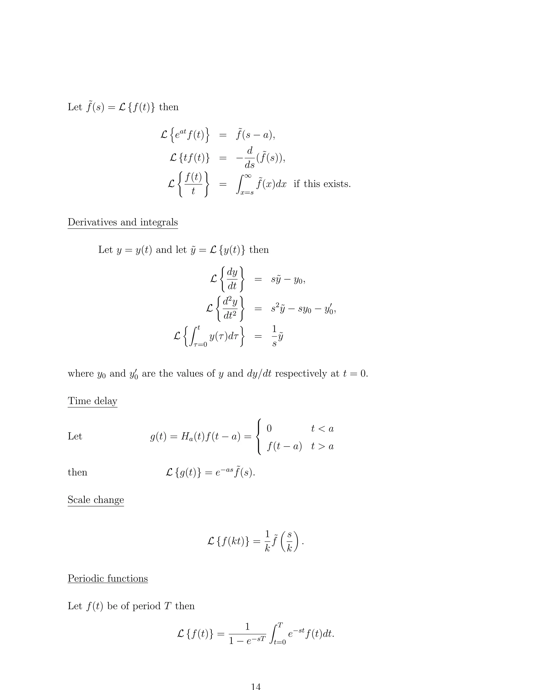
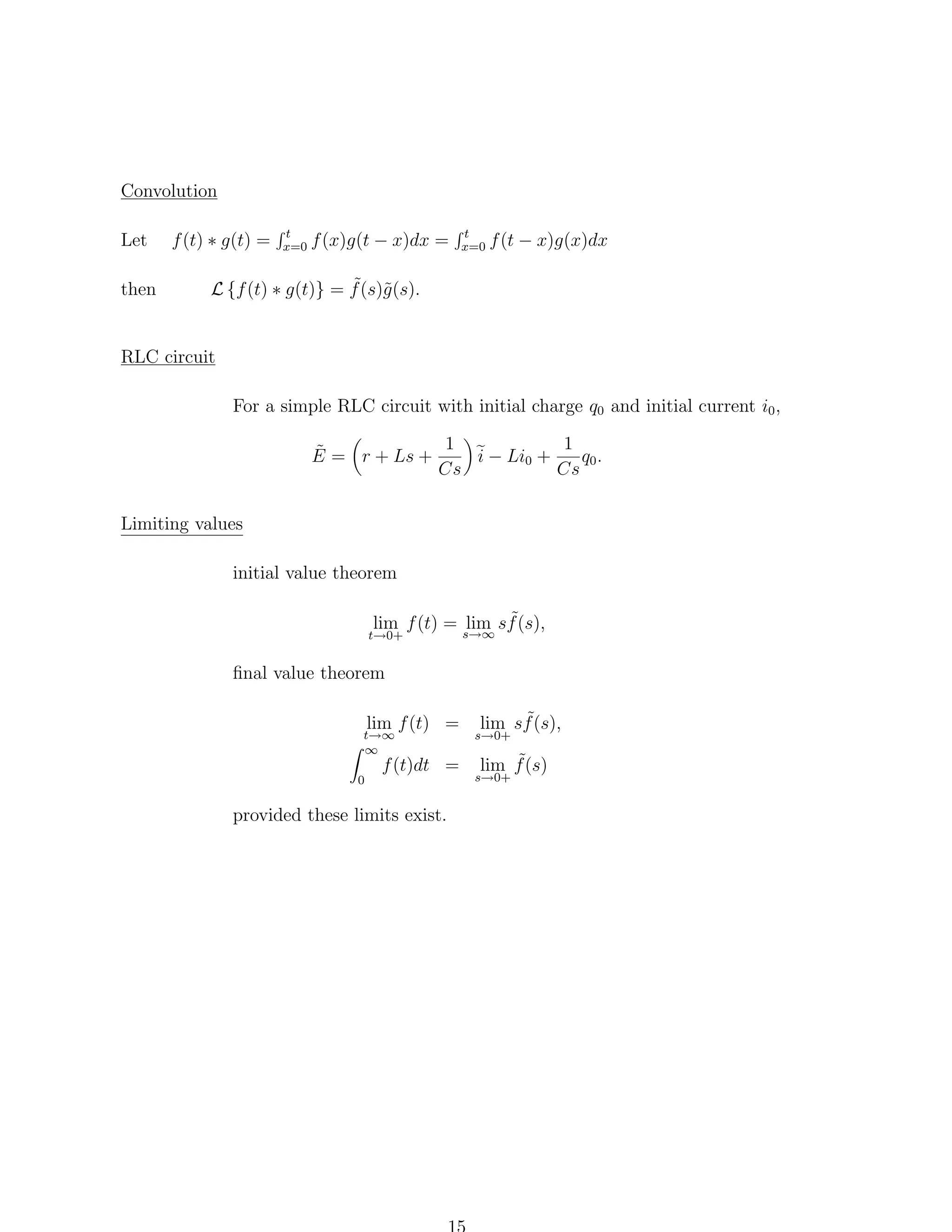
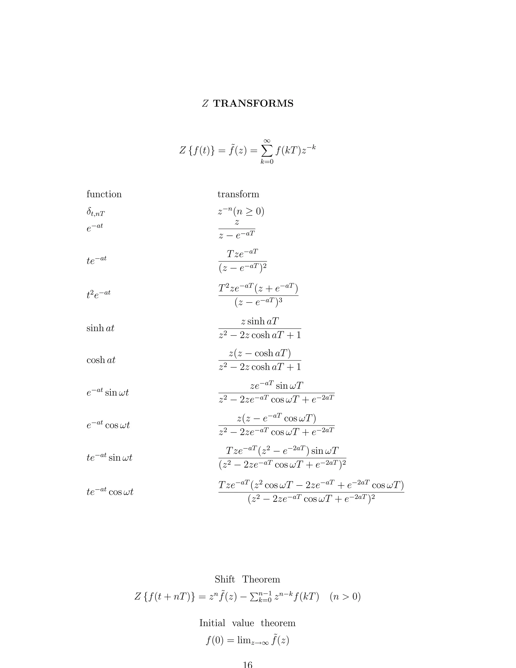
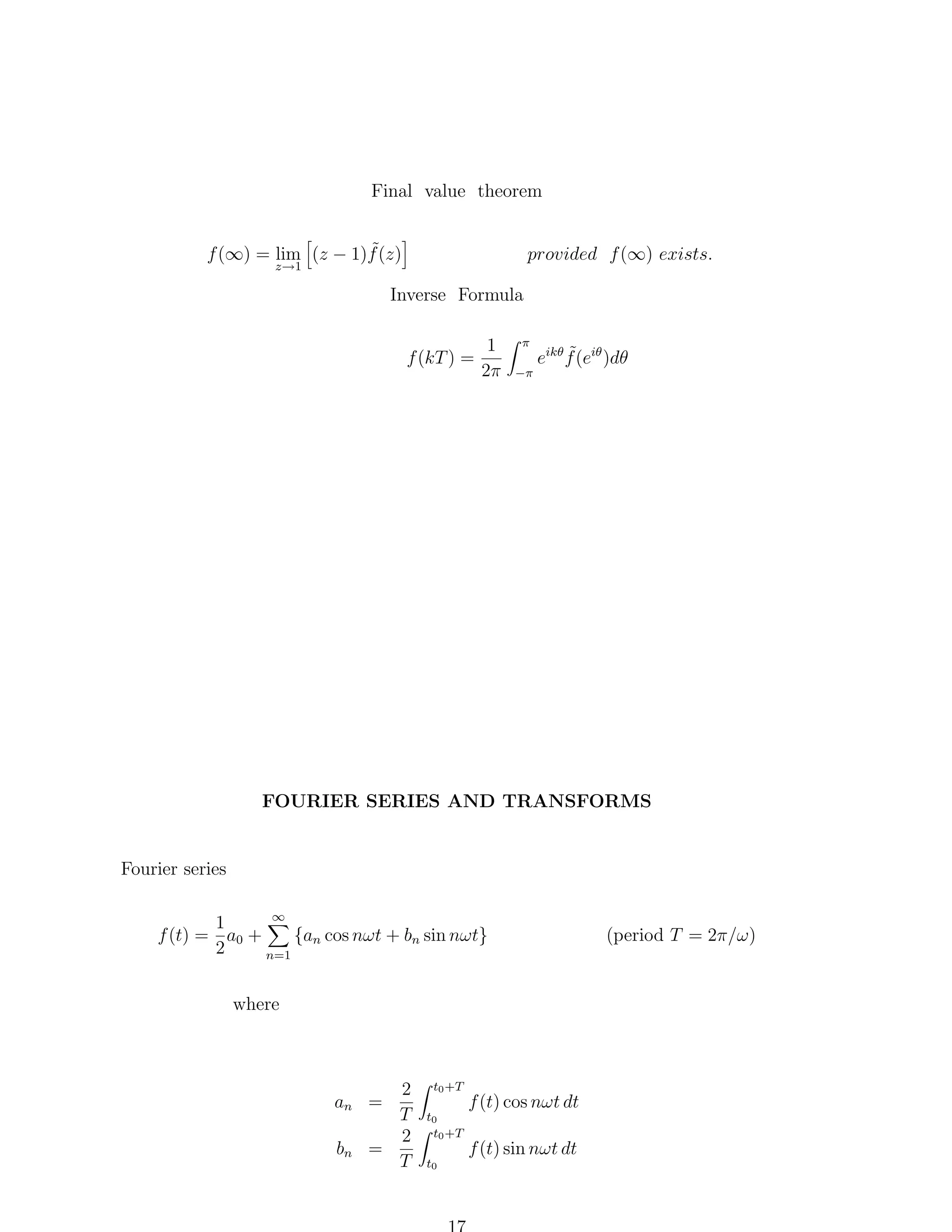
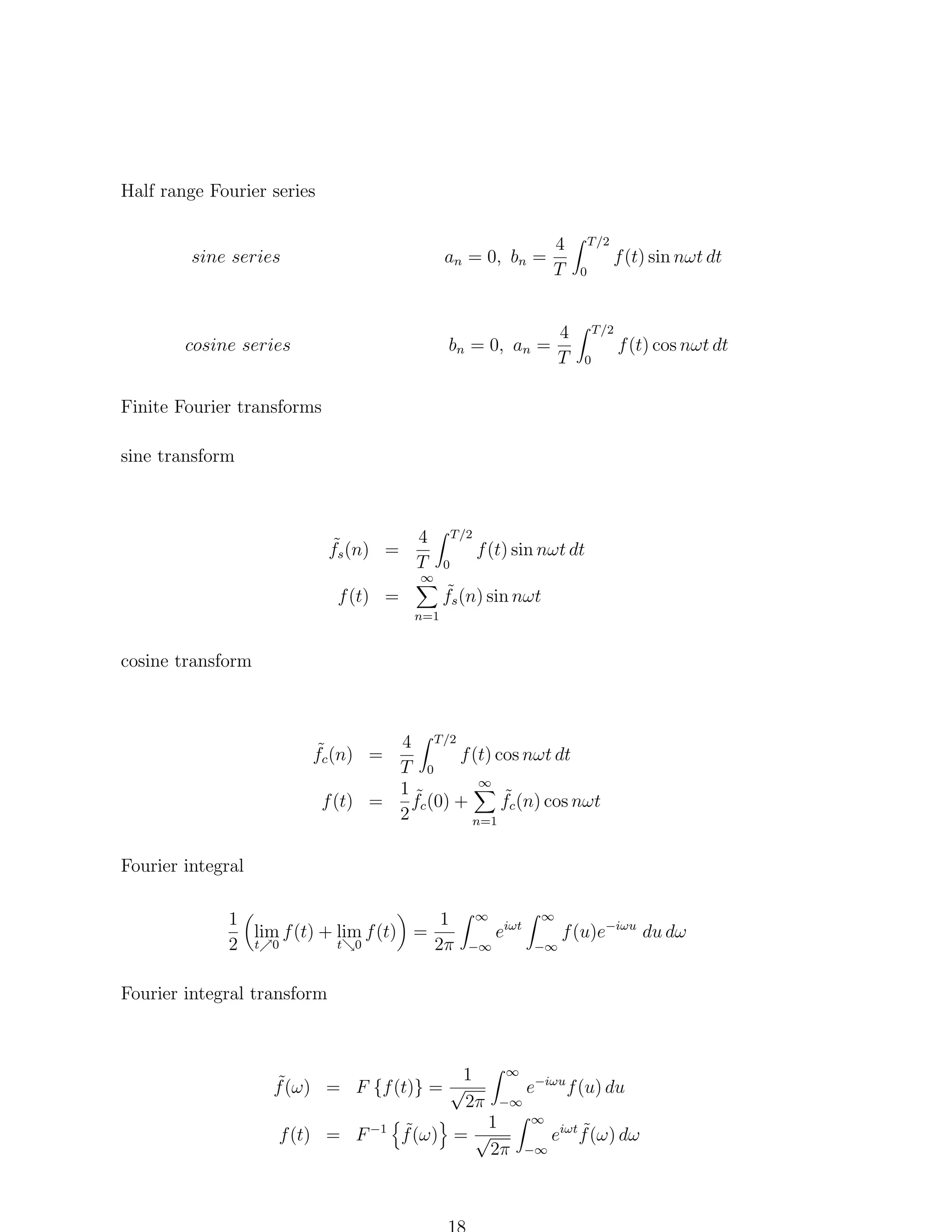
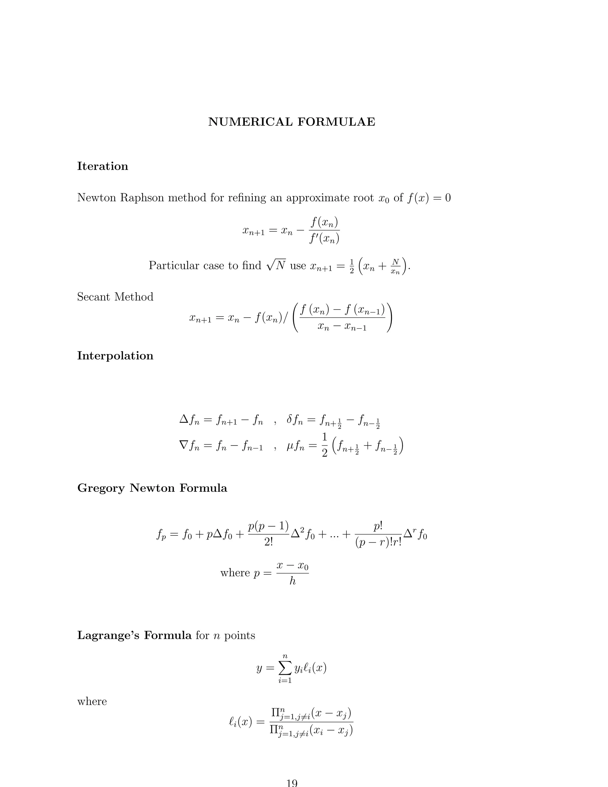
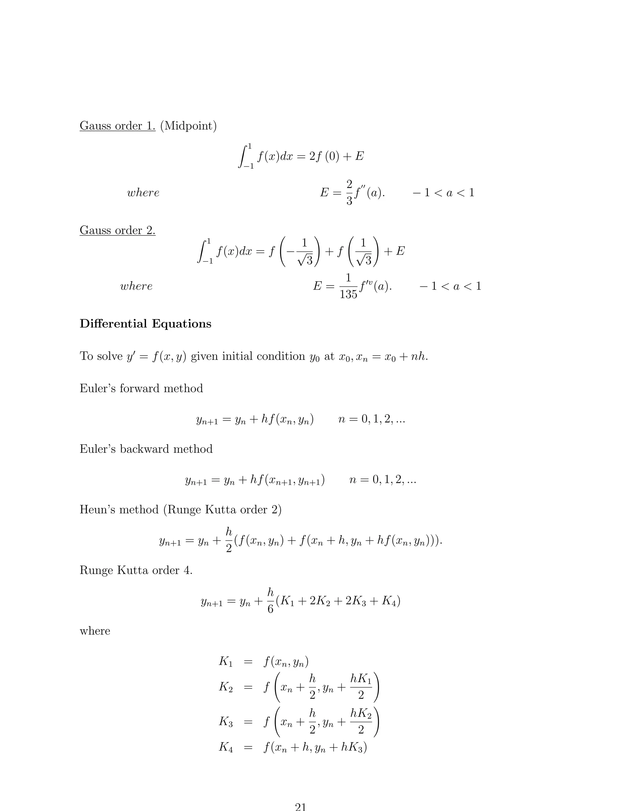
This document contains mathematical formula tables covering a wide range of topics including: - Greek alphabet - Indices and logarithms - Trigonometric, complex number, and hyperbolic identities - Power series expansions - Derivatives of common functions - Integrals of common functions - Laplace transforms - And more advanced topics such as vector calculus, mechanics, and statistical distributions.