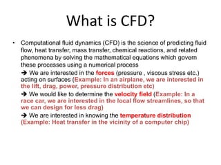
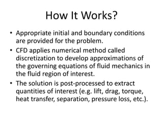
Computational fluid dynamics (CFD) is a numerical method used to analyze and solve fluid flow problems. CFD uses the mathematical equations that govern fluid motion and heat transfer to simulate the behavior of fluids. It provides a comprehensive examination of systems through modeling of velocity, pressure, temperature, and other properties without extensive physical testing. CFD has advantages of being relatively low cost, fast, and able to simulate real conditions. Limitations include accuracy depending on physical models and numerical errors from discretization. CFD is commonly used in engineering applications like aerodynamics, automotive, and electronics design.

1. CFD

2. What is CFD?
• Computational fluid dynamics (CFD) is the science of predicting fluid
flow, heat transfer, mass transfer, chemical reactions, and related
phenomena by solving the mathematical equations which govern
these processes using a numerical process
 We are interested in the forces (pressure , viscous stress etc.)
acting on surfaces (Example: In an airplane, we are interested in
the lift, drag, power, pressure distribution etc)
 We would like to determine the velocity field (Example: In a
race car, we are interested in the local flow streamlines, so that
we can design for less drag)
 We are interested in knowing the temperature distribution
(Example: Heat transfer in the vicinity of a computer chip)

3. Advantages
• Relatively low cost.
– CFD simulations are relatively inexpensive, and costs are
likely to decrease as computers become more powerful.
• Speed.
– CFD simulations can be executed in a short period of
time.
• Ability to simulate real conditions.
– CFD provides the ability to theoretically simulate any
physical condition.
• Comprehensive information.
– CFD allows the analyst to examine a large number of
locations in the region of interest, and yields a
comprehensive set of flow parameters for examination.

4. Limitations
• The CFD solutions can only be as accurate as the physical
models on which they are based.
• Solving equations on a computer invariably introduces
numerical errors.
– Round-off error: due to finite word size available on the
computer. Round-off errors will always exist (though they
can be small in most cases).
– Truncation error: due to approximations in the numerical
models. Truncation errors will go to zero as the grid is
refined. Mesh refinement is one way to deal with truncation
error.
• Boundary conditions.
– As with physical models, the accuracy of the CFD solution
is only as good as the initial/boundary conditions provided
to the numerical model.

5. Purpose and Aim
• Main purpose is Simulation-based design instead of “build & test”
hence saving a lot of time since it enables easy repetitions.
For example combustion explosions(unrepeatable).
• Aim is the simulation of physical fluid phenomena that are difficult for
experiments
– Full scale simulations (e.g., ships and airplanes)
– Environmental effects (wind, weather, etc.)
– Hazards (e.g., explosions, radiation, pollution)
– Physics (e.g., planetary boundary layer, stellar evolution)

6. How it works?
• Analysis begins with a mathematical model of a
physical problem.
• Conservation of matter, momentum, and energy
must be satisfied throughout the region of
interest.(Continuity, Momentum equation and
Energy equation).
• Fluid properties are modeled empirically.
• Simplifying assumptions are made in order to
make the problem tractable (e.g., steady-state,
incompressible, inviscid, two-dimensional etc.)

7. How It Works?
• Appropriate initial and boundary conditions
are provided for the problem.
• CFD applies numerical method called
discretization to develop approximations of
the governing equations of fluid mechanics in
the fluid region of interest.
• The solution is post-processed to extract
quantities of interest (e.g. lift, drag, torque,
heat transfer, separation, pressure loss, etc.).

8. Discretization
• Domain is discretized into a finite set of control volumes
or cells. The discretized domain is called the “grid” or the “mesh.”
• General conservation (transport) equations for mass, momentum,
energy, etc., are discretized into algebraic equations.
• All equations are solved to render flow field.
Fluid region of pipe flow discretized
into finite set of control volumes
(mesh).

9. Types Of Meshes
• Tri/tet vs. quad/hex meshes
• Hybrid mesh
Hybrid mesh for an IC
engine valve port
tet mesh
hex mesh
wedge mesh

10. Finite Volume Method Used In
Discretization
• The finite volume method (FVM) is a common approach used in CFD
codes, as it has an advantage in memory usage and solution speed,
especially for large problems, high Reynolds number turbulent flows,
and source term dominated flows (like combustion).
• In this method the governing partial differential equations are recast
in the conservative form and then solved over a discrete control
volumes and thus guarantees the conservation of fluxes through a
particular control volume.
• Here Q is the vector of conserved variables, F is the vector of
fluxes V is the volume of the control volume element, and A is the
surface area of the control volume element. The finite volume
equation yields governing equations in the form:

11. Finite element method
• The finite element method (FEM) is used in
structural analysis of solids, but is also
applicable to fluids.
• It is much more stable than the finite volume
approach. However, it can require more
memory and has slower solution than the
FVM.

12. Finite difference method
• The finite difference method (FDM) has
historical importance and is simple to
program.
• It is currently only used in few specialized
codes, which handle complex geometry with
high accuracy and efficiency by using
embedded boundaries or overlapping grids
(with the solution interpolated across each
grid).

13. Dinosaur mesh example

14. Examples:
The first figure shows the pressure fields on the given
layout
whereas the second one shows the velocity vectors

15. Numerical Model Setup
• For a given problem, you will need to:
– Select appropriate physical models.
– Define material properties.
• Fluid.
• Solid.
• Mixture.
– Prescribe operating conditions.
– Prescribe boundary conditions at all boundary
zones.
– Set up solver controls.
– Set up convergence monitors.

16. Calculation of Coefficient of Drag over
the Dinosaur
We calculate the theoretical values for the various parameters required for
calculation of the coefficient of drag on the dinosaur:
• Drag force: 17.4 N.
• Lift force: 5.5 N.
• Wind velocity: 5 m/s.
• Air density: 1.225 kg/m3.
• The dinosaur is 3.2 m tall.
• It has a projected frontal area of A = 2.91 m2.
• The drag coefficient is:
• This is pretty good compared to the average car! The streamlined back of the
dinosaur resulted in a flow pattern with very little separation.
11.0
91.2*25*225.1*5.0
4.17
2
2
1

Av
F
C D
D


17. Applications
Flow over F-16 at 45o angle of attack

18. Applications
• Flow over fixed wing – Expt. vs. CFD of
velocity contour

19. Applications
• Car safety thermal imaging using CFD
• Heat exchanger imaging
• Imaging of missile prototypes

20. Applications
• Electronics thermal analysis
• Designing of super duty vehicles like trucks ,
tempos etc.(based on thermal stress points)
• Thermal comfort in office environment