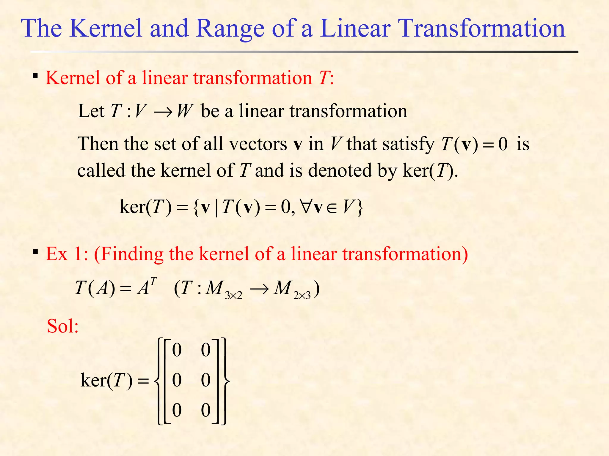
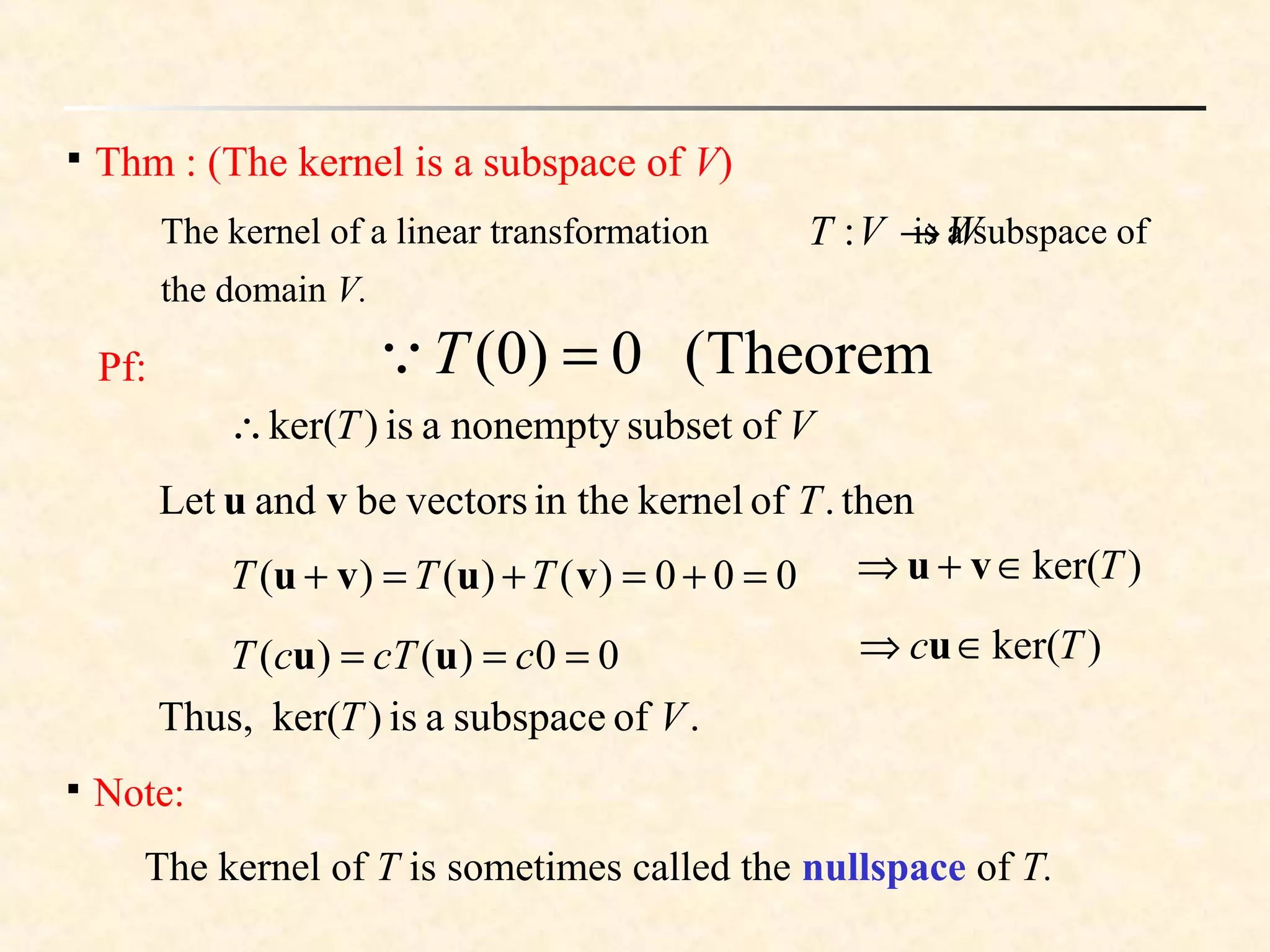
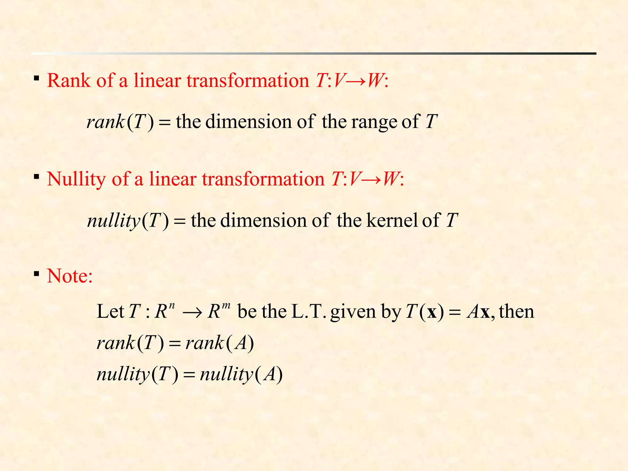
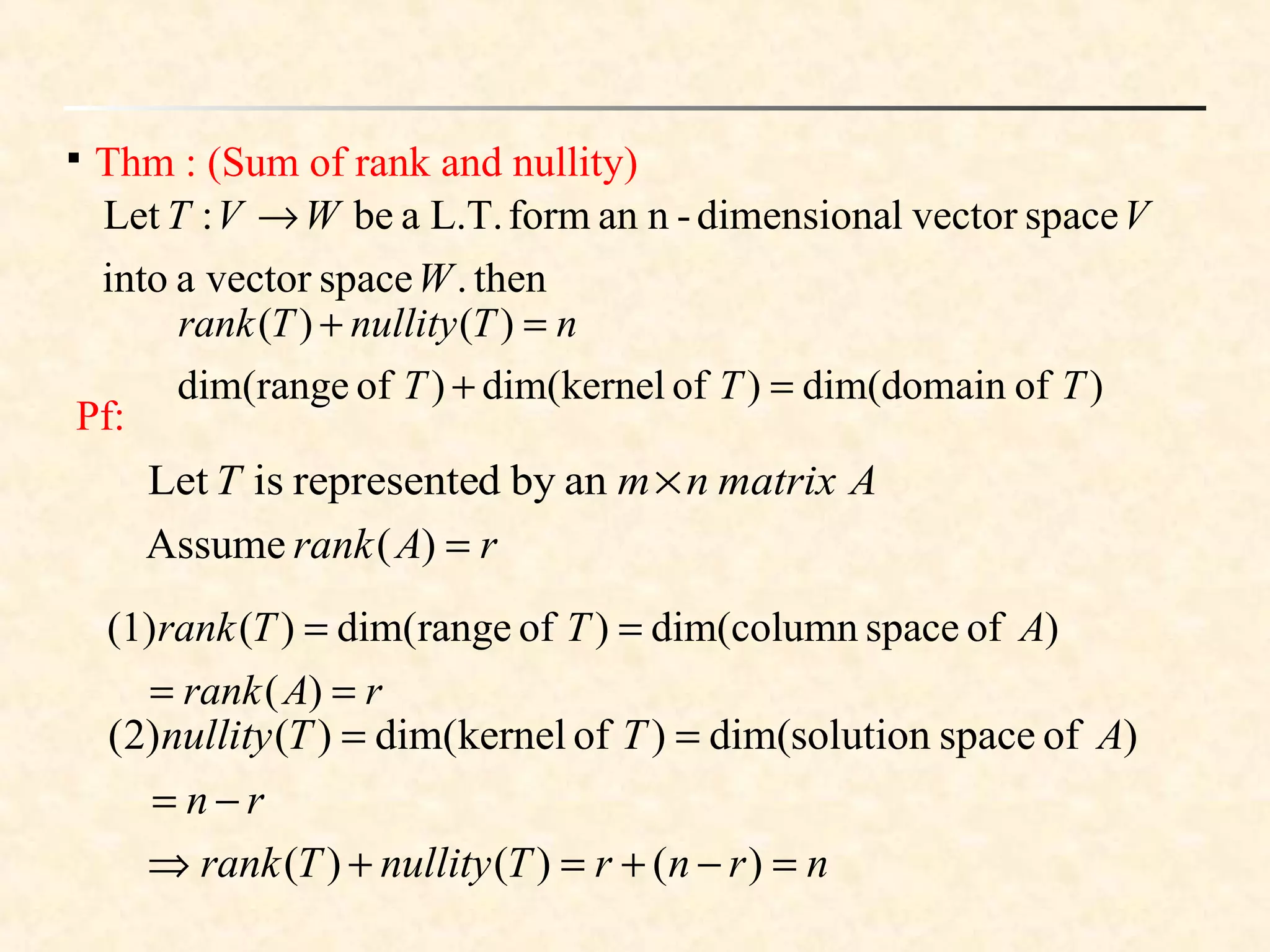
The document provides a comprehensive introduction to linear transformations, including their definitions, properties, kernels, ranges, and matrices associated with them. It also covers concepts like isomorphism, rank, nullity, and the relationship between linear transformations and matrices. Examples throughout the document illustrate these concepts in detail, aiding in understanding the mathematical principles involved.

1. 
VCLA

(Vector Calculus & Linear
Algebra )
Linear
Transformation
Guided by:-
Gayatri Mam
1/78
Sr no NAME ENROLL.NO.
1). Mansi Acharya 150450116001
2). Drashti Patel 150450116024
3). Jyoti Mishra 150450116018
MADE BY:-

2. CONTENTS
 Introduction to Linear Transformations
 The Kernel and Range of a Linear Transformation
 Matrices for Linear Transformations
 Transition Matrices and Similarity

3. Introduction to Linear Transformations

Function T that maps a vector space V into a vector space W:
spacevector:,,: mapping
WVWVT  →
V: the domain of T
W: the codomain of T

4. 
Image of v under T:
If v is in V and w is in W such that
wv =)(T
Then w is called the image of v under T .

the range of T:
The set of all images of vectors in V.

the preimage of w:
The set of all v in V such that T(v)=w.

5. 
Ex 1: (A function from R2
into R2
)
22
: RRT →
)2,(),( 212121 vvvvvvT +−=
2
21 ),( Rvv ∈=v
(a) Find the image of v=(-1,2). (b) Find the preimage of w=(-1,11)
Sol:
)3,3())2(21,21()2,1()(
)2,1()(
−=+−−−=−=⇒
−=
TT
a
v
v
)11,1()()( −== wvTb
)11,1()2,(),( 212121 −=+−= vvvvvvT
112
1
21
21
=+
−=−⇒
vv
vv
4,3 21 ==⇒ vv Thus {(3, 4)} is the preimage of w=(-1,
11).

6. 
Linear Transformation (L.T.):
nnsformatiolinear trato：:
spacevector：,
WVWVT
WV
→
VTTT ∈∀+=+ vuvuvu ,),()()((1)
RccTcT ∈∀= ),()()2( uu

7. 
Notes:
(1) A linear transformation is said to be operation preserving.
)()()( vuvu TTT +=+
Addition
in V
Addition
in W
)()( uu cTcT =
Scalar
multiplication
in V
Scalar
multiplication
in W
(2) A linear transformation from a vector space into itself
is called a linear operator.
VVT →:

8. ),(),(
tionmultiplicaScalar)2(
2121 cucuuucc ==u
)(
)2,(
)2,(),()(
2121
212121
u
u
cT
uuuuc
cucucucucucuTcT
=
+−=
+−==
Therefore, T is a linear transformation.

9. 
Notes: Two uses of the term “linear”.
(1) is called a linear function because its graph is a
line.
1)( += xxf
(2) is not a linear transformation from a vector
space R into R because it preserves neither vector
addition nor scalar multiplication.
1)( += xxf

10. 
Zero transformation:
VWVT ∈→ vu,,:
VT ∈∀= vv ,0)(

Identity transformation:
VVT →: VT ∈∀= vvv ,)(

Thm : (Properties of linear transformations)
WVT →:
00 =)((1)T
)()((2) vv TT −=−
)()()((3) vuvu TTT −=−
)()()(
)()(Then
If(4)
2211
2211
2211
nn
nn
nn
vTcvTcvTc
vcvcvcTT
vcvcvc
+++=
+++=
+++=



v
v

11. 
Thm : (The linear transformation given by a matrix)
Let A be an m×n matrix. The function T defined by
vv AT =)(
is a linear transformation from Rn
into Rm
.

Note:












+++
+++
+++
=
























=
nmnmm
nn
nn
nmnmm
n
n
vavava
vavava
vavava
v
v
v
aaa
aaa
aaa
A









2211
2222121
1212111
2
1
21
22221
11211
v
vv AT =)(
mn
RRT →:
vectorn
R vectorm
R

12. The Kernel and Range of a Linear Transformation

Kernel of a linear transformation T:
Let be a linear transformationWVT →:
Then the set of all vectors v in V that satisfy is
called the kernel of T and is denoted by ker(T).
0)( =vT
},0)(|{)ker( VTT ∈∀== vvv

Ex 1: (Finding the kernel of a linear transformation)
):()( 3223 ×× →= MMTAAT T
Sol:




















=
00
00
00
)ker(T

13. 
Thm : (The kernel is a subspace of V)
The kernel of a linear transformation is a subspace of
the domain V.
WVT →:
Pf:
VT ofsubsetnonemptyais)ker(∴
then.ofkernelin thevectorsbeandLet Tvu
000)()()( =+=+=+ vuvu TTT
00)()( === ccTcT uu )ker(Tc ∈⇒ u
)ker(T∈+⇒ vu
.ofsubspaceais)ker(Thus, VT

Note:
The kernel of T is sometimes called the nullspace of T.
Theorem(0)0( =T

14. 
Rank of a linear transformation T:V→W:
TTrank ofrangetheofdimensionthe)( =

Nullity of a linear transformation T:V→W:
TTnullity ofkerneltheofdimensionthe)( =

Note:
)()(
)()(
then,)(bygivenL.T.thebe:Let
AnullityTnullity
ArankTrank
ATRRT mn
=
=
=→ xx

15. then.spacevectorainto
spacevectorldimensiona-nanformL.T.abe:Let
W
VWVT →

Thm : (Sum of rank and nullity)
Pf:
AmatrixnmT anbydrepresenteisLet ×
)ofdomaindim()ofkerneldim()ofrangedim(
)()(
TTT
nTnullityTrank
=+
=+
rArank =)(Assume
rArank
ATTrank
==
==
)(
)ofspacecolumndim()ofrangedim()((1)
nrnrTnullityTrank =−+=+⇒ )()()(
rn
ATTnullity
−=
== )ofspacesolutiondim()ofkerneldim()()2(

16. 
Isomorphism:
other.eachtoisomorphicbetosaidare
andthen,tofrommisomorphisanexiststheresuch that
spacesvectorareandifMoreover,m.isomorphisancalledis
ontoandonetooneisthat:nnsformatiolinear traA
WVWV
WV
WVT →

Thm : (Isomorphic spaces and dimension)
Pf:
.dimensionhaswhere,toisomorphicisthatAssume nVWV
onto.andonetooneisthat:L.T.aexistsThere WVT →⇒
one-to-oneisT
nnTKerTT
TKer
=−=−=⇒
=⇒
0))(dim()ofdomaindim()ofrangedim(
0))(dim(
Two finite-dimensional vector space V and W are isomorphic
if and only if they are of the same dimension.

17. .dimensionhavebothandthatAssume nWV
onto.isT
nWT ==⇒ )dim()ofrangedim(
nWV == )dim()dim(Thus
{ }
{ } .ofbasisabe,,,let
andV,ofbasisabe,,,Let
21
21
Wwww
vvv
n
n


nnvcvcvc
V
+++= 2211
asdrepresentebecaninvectorarbitraryanThen
v
nnwcwcwcT
WVT
+++=
→
2211)(
follows.as:L.T.adefinecanyouand
v
It can be shown that this L.T. is both 1-1 and onto.
Thus V and W are isomorphic.

18. Matrices for Linear Transformations
)43,23,2(),,()1( 32321321321 xxxxxxxxxxxT +−+−−+=

Three reasons for matrix representation of a linear transformation:
















−−
−
==
3
2
1
430
231
112
)()2(
x
x
x
AT xx

It is simpler to write.

It is simpler to read.

It is more easily adapted for computer use.

Two representations of the linear transformation T:R3
→R3
:

19. 
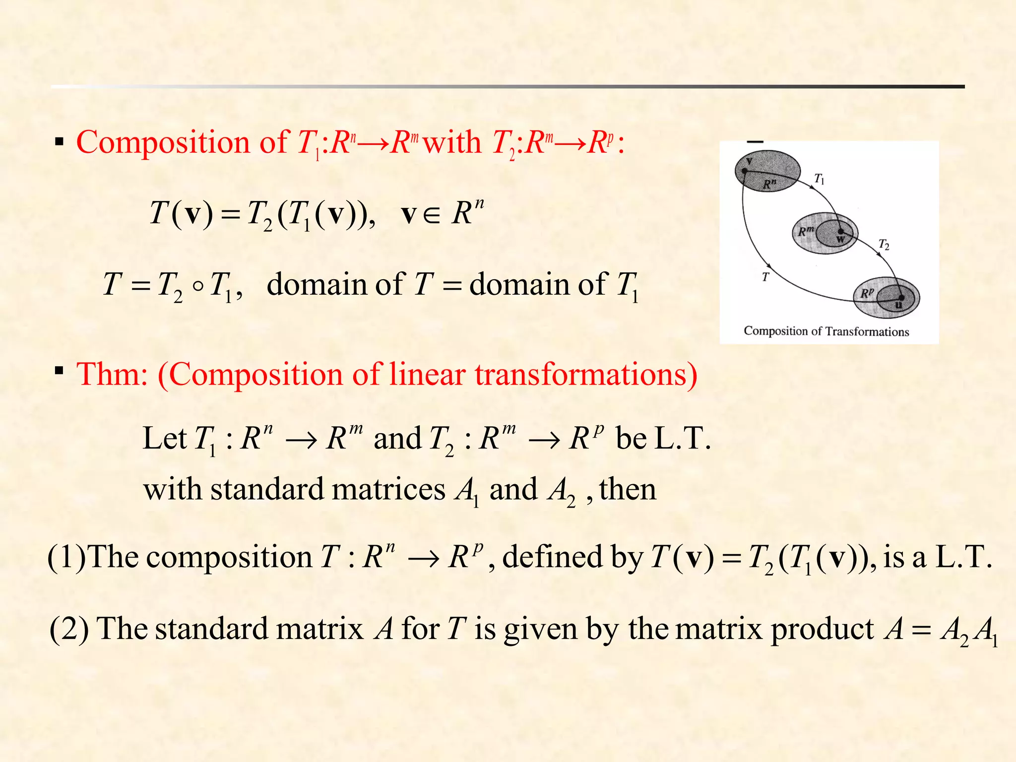
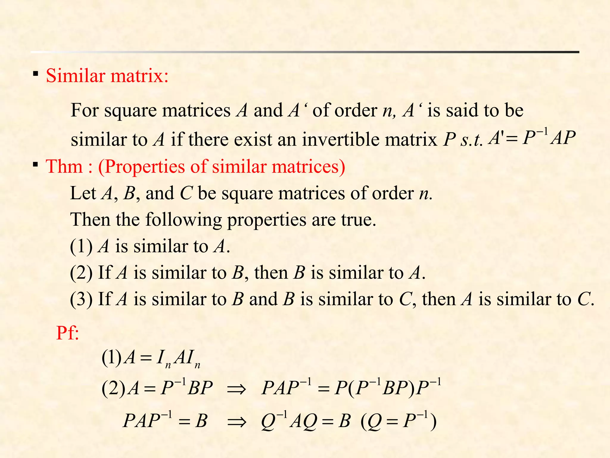
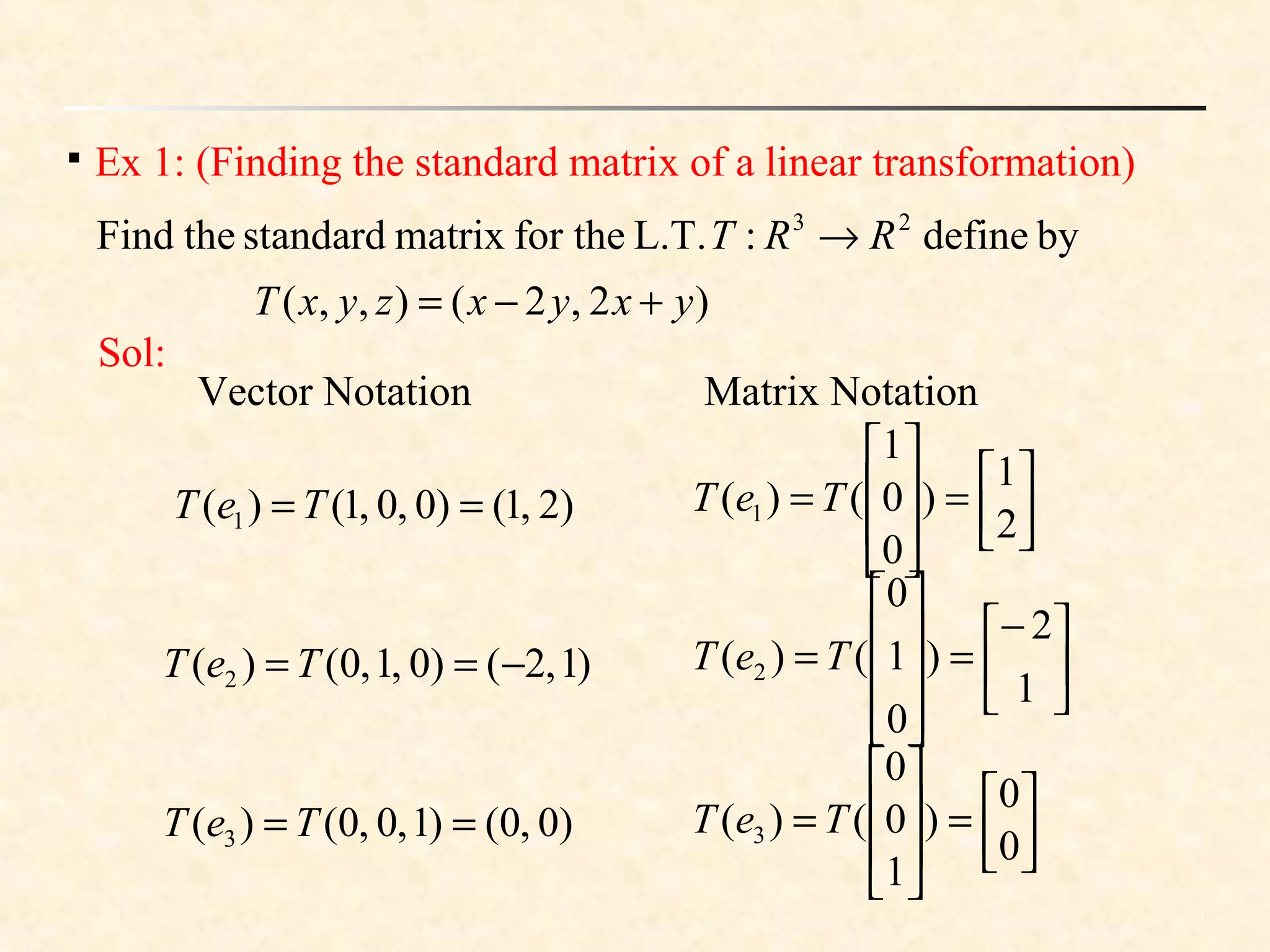
Thm : (Standard matrix for a linear transformation)
such thatonansformatilinear trtabe:Let mn
RRT →
,)(,,)(,)( 2
1
2
22
12
2
1
21
11
1












=












=












=
mn
n
n
n
mm a
a
a
eT
a
a
a
eT
a
a
a
eT



)(tocorrespondcolumnssematrix whoThen the i
eTnnm×
.formatrixstandardthecalledisA
.ineveryfor)(such thatis
T
RAT n
vvv =
[ ]












==
mnmm
n
n
n
aaa
aaa
aaa
eTeTeTA





21
22221
11211
21 )()()(

20. 
Ex 1: (Finding the standard matrix of a linear transformation)
bydefine:L.T.for thematrixstandardtheFind 23
RRT →
)2,2(),,( yxyxzyxT +−=
Sol:
)2,1()0,0,1()( 1 == TeT
)1,2()0,1,0()( 2 −== TeT
)0,0()1,0,0()( 3 == TeT
2
1
)
0
0
1
()( 1 



=








= TeT
1
2
)
0
1
0
()( 2 




−
=










= TeT
0
0
)
1
0
0
()( 3 



=








= TeT
Vector Notation Matrix Notation

21.  Composition of T1:Rn
→Rm
with T2:Rm
→Rp
:
n
RTTT ∈= vvv )),(()( 12
112 ofdomainofdomain, TTTTT == 

Thm: (Composition of linear transformations)
then,andmatricesstandardwith
L.T.be:and:Let
21
21
AA
RRTRRT pmmn
→→
L.T.ais)),(()(bydefined,:ncompositioThe(1) 12 vv TTTRRT pn
=→
12productmatrixby thegivenisformatrixstandardThe)2( AAATA =

22. 
Inverse linear transformation:
ineveryfors.t.L.T.are:and:If 21
nnnnn
RRRTRRT v→→
))((and))(( 2112 vvvv == TTTT
invertiblebetosaidisandofinversethecalledisThen 112 TTT

Note:
If the transformation T is invertible, then the inverse is
unique and denoted by T–1
.

23. 
the matrix of T relative to the bases B and B':
)forbasis(a},,,{'
)forbasis(a},,,{
)L.T.a(:
21
21
WwwwB
VvvvB
WVT
m
n


=
=
→
Thus, the matrix of T relative to the bases B and B' is
[ ] [ ] [ ][ ] nmBnBB
MvTvTvTA ×∈= ''2'1 )(,,)(,)( 

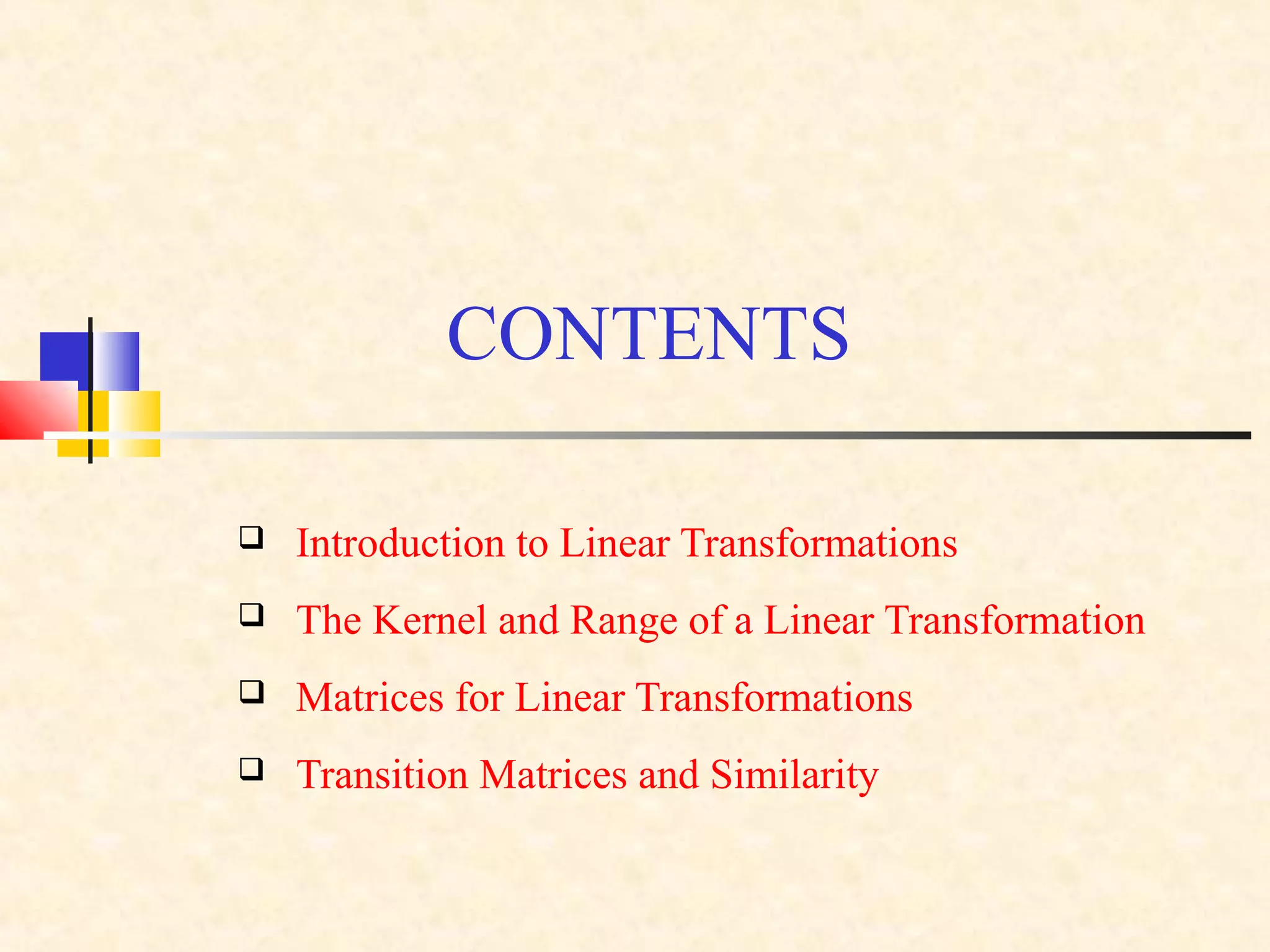
24. Transition Matrices and Similarity
)ofbasis(a},,,{'
)ofbasisa(},,,{
)L.T.a(:
21
21
VwwwB
VvvvB
VVT
n
n


=
=
→
[ ] [ ] [ ][ ] )torelativeofmatrix()(,,)(,)( 21 BTvTvTvTA BnBB
=
[ ] [ ] [ ][ ] )'torelativeof(matrix)(,,)(,)(' ''2'1 BTwTwTwTA BnBB
=
[ ] [ ] [ ][ ] )to'frommatrixntransitio(,,, 21 BBwwwP BnBB
=
[ ] [ ] [ ][ ] )'tofrommatrixntransitio(,,, ''2'1
1
BBvvvP BnBB
=−
[ ] [ ] [ ] [ ]BBBB PP vvvv 1
'', −
==∴
[ ] [ ]
[ ] [ ] '' ')(
)(
BB
BB
AT
AT
vv
vv
=
=

25. 
Two ways to get from to :
'' )]([]['
)direct)(1(
BB TA vv =
[ ] 'Bv [ ] ')( BT v
''
1
)]([][
(indirect))2(
BB TAPP vv =−
APPA 1
' −
=⇒
direct
indirect

26. 
Similar matrix:
For square matrices A and A‘ of order n, A‘ is said to be
similar to A if there exist an invertible matrix P s.t. APPA 1
' −
=

Thm : (Properties of similar matrices)
Let A, B, and C be square matrices of order n.
Then the following properties are true.
(1) A is similar to A.
(2) If A is similar to B, then B is similar to A.
(3) If A is similar to B and B is similar to C, then A is similar to C.
Pf:
nn AIIA =)1(
)(
)()2(
111
1111
−−−
−−−−
==⇒=
=⇒=
PQBAQQBPAP
PBPPPPAPBPPA