Downloaded 76 times

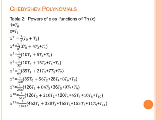
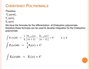
![CHEBYSHEV POLYNOMIALS
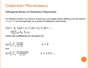
In mathematics the Chebyshev polynomials, named after Pafnuty Chebyshev,[1] are a sequence
of orthogonal polynomials which are related to de Moivre's formula and which can be defined
recursively. One usually distinguishes between Chebyshev polynomials of the first kind which
are denoted Tn and Chebyshev polynomials of the second kind which are denoted Un. The letter
T is used because of the alternative transliterations of the name Chebyshev as T chebycheff, T
chebyshev (French) or T schebyschow (German).
The Chebyshev polynomials Tn or Un are polynomials of degree n and the sequence of
Chebyshev polynomials of either kind composes a polynomial sequence.
Chebyshev polynomials are polynomials with the largest possible leading coefficient, but
subject to the condition that their absolute value on the interval [-1,1] is bounded by 1. They
are also the extremal polynomials for many other properties.[2]
Chebyshev polynomials are important in approximation theory because the roots of the
Chebyshev polynomials of the first kind, which are also called Chebyshev nodes, are used as
nodes in polynomial interpolation. The resulting interpolation polynomial minimizes the
problem of Runge's phenomenon and provides an approximation that is close to the
polynomial of best approximation to a continuous function under the maximum norm. This
approximation leads directly to the method of Clenshaw–Curtis quadrature.](https://image.slidesharecdn.com/presentationmathmatic3-151224175058/85/Presentation-mathmatic-3-3-320.jpg)
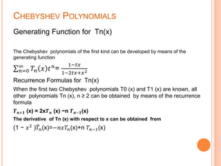
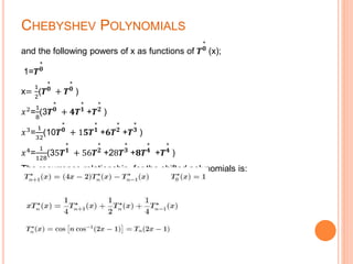
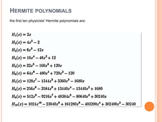
![CHEBYSHEV POLYNOMIALS
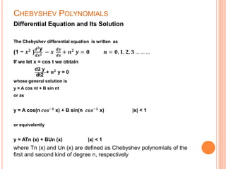
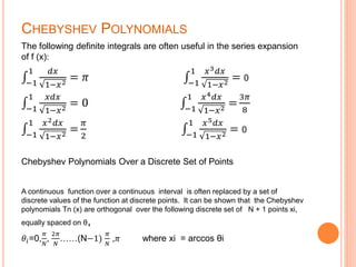
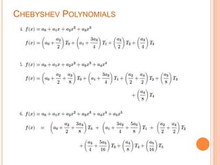
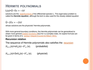
from which we obtain
𝑻 𝒏 (x)=
𝟏
𝟐
[( x +i 𝟏 − 𝒙 𝟐) 𝒏
+ ( x − i 𝟏 − 𝒙 𝟐) 𝒏
]
For |x| > 1 we have
Tn (x) + Un (x) = 𝒆 𝒏𝒕
= (x± 𝟏 − 𝒙 𝟐) 𝒏
Tn (x) − Un (x) = 𝒆−𝒏𝒕
= (x± 𝟏 − 𝒙 𝟐) 𝒏
The sum of the last two relationships give the same result for Tn (x).
Chebyshev Polynomials of the First Kind of Degree n
The Chebyshev polynomials Tn (x) can be obtained by means of
Rodrigue’s formula
𝑻 𝒏 (x)=
(−𝟐) 𝒏 𝒏!
𝟐𝒏!
𝟏 − 𝒙 𝟐 𝒅 𝒏
𝒅𝒙 𝒏(1-𝒙 𝟐) 𝒏−𝟏/𝟐 n=0,1,2,3,……….](https://image.slidesharecdn.com/presentationmathmatic3-151224175058/85/Presentation-mathmatic-3-6-320.jpg)
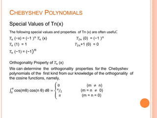
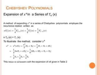
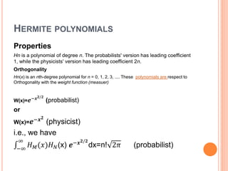
![CHEBYSHEV POLYNOMIALS
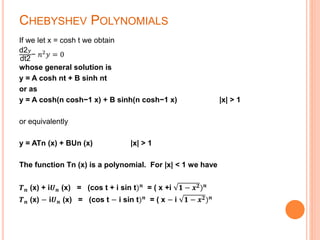
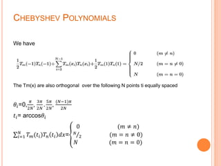
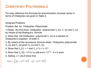
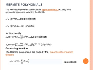
The set of points ti are clearly the midpoints in θ of the first case. The unequal
spacing of the points in xi(N ti) compensates for the weight factor
W(x)= (1 − 𝑥2
)
−1
2
in the continuous case.
Additional Identities of Chebyshev Polynomials
The Chebyshev polynomials are both orthogonal polynomials and the trigonometric
cos nx functions in disguise, therefore they satisfy a large number of useful
relationships.
The differentiation and integration properties are very important in analytical and
numerical work. We begin with
𝑇𝑛+1 (x) = cos[(n + 1) 𝑐𝑜𝑠−1
x]
and
𝑇𝑛−1 (x) = cos[(n - 1) 𝑐𝑜𝑠−1 x]](https://image.slidesharecdn.com/presentationmathmatic3-151224175058/85/Presentation-mathmatic-3-15-320.jpg)

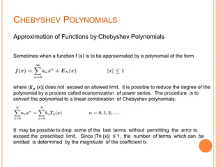
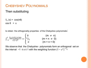
![CHEBYSHEV POLYNOMIALS
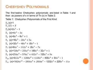
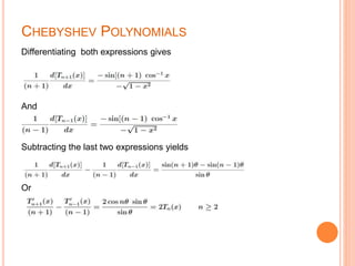
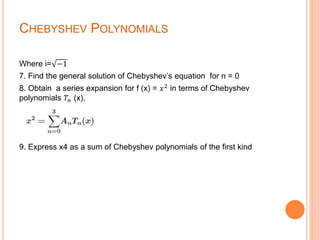
The Chebyshev polynomials are useful in numerical work for the interval −1
≤ x ≤ 1 because
1. |Tn (x)] ≤ 1 within −1 ≤ x ≤ 1
2. The maxima and minima are of comparable value
3. The maxima and minima are spread reasonably uniformly over the interval −1
≤ x ≤ 1
4. All Chebyshev polynomials satisfy a three term recurrence relation
5. They are easy to compute and to convert to and from a power series form.
These properties together produce an approximating polynomial which
minimizes error in its application. This is different from the least squares
approximation where the sum of the squares of the errors is minimized; the
maximum error itself can be quite large. In the Chebyshev approximation,
the average error can be large but the maximum error is minimized.
Chebyshev approximations of a function are sometimes said to be mini-max
approximations of the function.](https://image.slidesharecdn.com/presentationmathmatic3-151224175058/85/Presentation-mathmatic-3-22-320.jpg)


The document discusses Chebyshev polynomials. It defines Chebyshev polynomials as orthogonal polynomials related to de Moivre's formula that can be defined recursively. It provides key properties of Chebyshev polynomials including that they are the extremal polynomials for many properties and important in approximation theory. The document also provides formulas for generating Chebyshev polynomials, their orthogonality properties, and their use in representing functions through orthogonal series expansions.