Downloaded 643 times

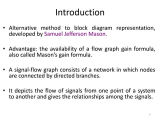
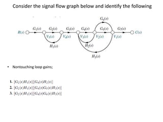
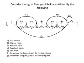
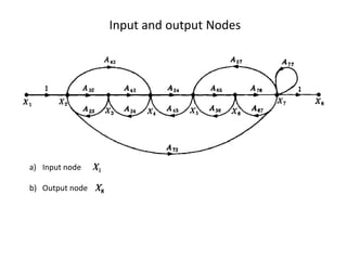
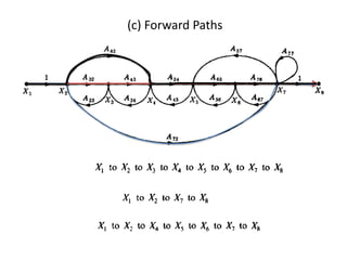
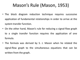
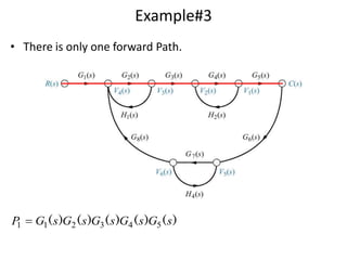
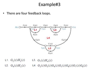
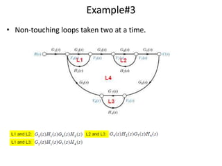
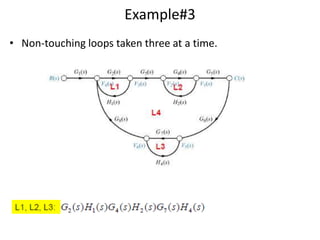


This document provides an overview of signal flow graphs including: - Definitions and terminology of signal flow graphs - Examples of constructing signal flow graphs from equations and block diagrams - Mason's gain formula for calculating the transfer function of a system from its signal flow graph representation in 3 sentences or less - Examples are provided to demonstrate applying Mason's gain formula to calculate transfer functions from given signal flow graphs.


![Reduction of multiple subsystem [compatibility mode]](https://cdn.slidesharecdn.com/ss_thumbnails/reductionofmultiplesubsystemcompatibilitymode-110418075355-phpapp01-thumbnail.jpg?width=640&height=640&fit=bounds)