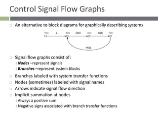
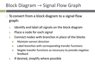
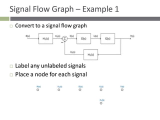
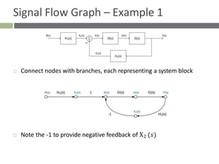
Signal flow graphs consist of: 🞑 Nodes –represent signals 🞑 Branches –represent system blocks Branches labeled with system transfer functions

1. Control Signal Flow Graphs
 An alternative to block diagrams for graphically describing systems
 Signal flow graphs consist of:
🞑 Nodes –represent signals
🞑 Branches –represent system blocks
 Branches labeled with system transfer functions
 Nodes (sometimes) labeled with signal names
 Arrows indicate signal flow direction
 Implicit summation at nodes
🞑 Always a positive sum
🞑 Negative signs associated with branch transfer functions

2. Block Diagram → Signal Flow Graph
 Toconvert from a block diagram to a signal flow
graph:
1. Identify and label all signals on the block diagram
2. Place a node for each signal
3. Connect nodes with branches in place of the blocks
 Maintain correct direction
 Label branches with corresponding transfer functions
 Negate transfer functions as necessary to provide negative
feedback
4. If desired, simplify where possible

3. Signal Flow Graph – Example 1
 Convert to a signal flow graph
 Label any unlabeled signals
 Place a node for each signal

4. Signal Flow Graph – Example 1
 Connect nodes with branches, each representing a system block
 Note the -1 to provide negative feedback of X2 𝑠

5. Signal Flow Graph – Example 1
 Nodes with a single input and single output can be
eliminated, if desired
🞑 This makes sense for X1 𝑠 and X2 𝑠
🞑 Leave 𝑈 𝑠 to indicate separation between controller and plant

6. Signal Flow Graph – Example 2
 Revisit the block diagram from earlier
🞑 Convert to a signal flow graph
 Label all signals, then place a node for each

7. Signal Flow Graph – Example 2
 Connect nodes with branches

8. Signal Flow Graph – Example 2
 Simplify – eliminate X5 𝑠 , X6 𝑠 , X7 𝑠 , and X8 𝑠

9. 40
Mason’s Rule
 We’ve seen how to reduce a complicated block
diagram to a single input-to-output transfer
function
🞑 Many successive simplifications
 Mason’s rule provides a formula to calculate the
same overall transfer function
🞑 Single application of the formula
🞑 Can get complicated
 Before presenting the Mason’s rule formula, we
need to define some terminology

10. 41
Loop Gain
 Loop gain – total gain (product of individual gains) around
any path in the signal flow graph
🞑 Beginning and ending at the same node
🞑 Not passing through any node more than once
 Here, there are three loops with the following gains:
1. −𝐺1𝐻3
2. 𝐺2𝐻1
3. −𝐺2𝐺3𝐻2

11. 42
Forward Path Gain
 Forward path gain – gain along any path from the input
to the output
🞑 Not passing through any node more than once
 Here, there are two forward paths with the following
gains:
1. 𝐺1𝐺2𝐺3𝐺4
2. 𝐺1𝐺2𝐺5

12. 43
Non-Touching Loops
 Non-touching loops – loops that do not have any
nodes in common
 Here,
1. −𝐺1𝐻3 does not touch 𝐺2𝐻1
2. −𝐺1𝐻3 does not touch −𝐺2𝐺3𝐻2

13. 44
Non-Touching Loop Gains
 Non-touching loop gains – the product of loop gains
from non-touching loops, taken two, three, four, or
more at a time
 Here, there are only two pairs of non-touching loops
1.
2.
−𝐺1𝐻3 ⋅ 𝐺2𝐻1
−𝐺1𝐻3 ⋅ −𝐺2𝐺3𝐻2

14. 45
Mason’s Rule
𝑇 𝑠
𝑃
𝑌 𝑠 1
= = � 𝑇𝑘Δ𝑘
𝑅 𝑠 Δ
𝑘=1
where
𝑃 = # of forward paths
𝑇𝑘 = gain of the 𝑘𝑡ℎ forward path
Δ = 1 − Σ(loop gains)
+Σ(non-touching loop gains taken two-at-a-time)
−Σ(non-touching loop gains taken three-at-a-time)
+Σ(non-touching loop gains taken four-at-a-time)
−Σ …
Δ𝑘 = Δ − Σ(loop gain terms in Δ that touch the 𝑘𝑡ℎ forward path)

15. 46
Mason’s Rule - Example
 # of forward paths:
𝑃 = 2
 Forward path gains:
𝑇1= 𝐺1𝐺2𝐺3𝐺4
𝑇2 = 𝐺1𝐺2𝐺5
 Σ(loop gains):
−𝐺1𝐻3 + 𝐺2𝐻1 − 𝐺2𝐺3𝐻2
 Σ(NTLGs taken two-at-a-time):
−𝐺1𝐻3𝐺2𝐻1 + 𝐺1𝐻3𝐺2𝐺3𝐻2
 Δ:
Δ = 1 − −𝐺1𝐻3 + 𝐺2𝐻1 − 𝐺2𝐺3𝐻2
+ −𝐺1𝐻3𝐺2𝐻1 + 𝐺1𝐻3𝐺2𝐺3𝐻2

16. 47
Mason’s Rule – Example - Δ𝑘
 Simplest way to find Δ𝑘 terms is to calculate Δ with the 𝑘𝑡ℎ
path removed – must remove nodes as well
 𝑘 = 1:
 With forward path 1 removed, there are no loops, so
Δ1 = 1 − 0
Δ1 = 1

17. 48
Mason’s Rule – Example - Δ𝑘
 𝑘 = 2:
 Similarly, removing forward path 2 leaves no loops, so
Δ2 = 1 − 0
Δ2 = 1

18. 49
Mason’s Rule - Example
 For our example:
𝑃 = 2
𝑇1= 𝐺1𝐺2𝐺3𝐺4
𝑇2 = 𝐺1𝐺2𝐺5
Δ = 1 + 𝐺1𝐻3 − 𝐺2𝐻1 + 𝐺2𝐺3𝐻2 − 𝐺1𝐻3𝐺2𝐻1 + 𝐺1𝐻3𝐺2𝐺3𝐻2
Δ1 = 1
Δ2 = 1
 The closed-loop transfer function:
𝑇 𝑠
𝑇1Δ1 + 𝑇2Δ2
=
Δ
𝑇 𝑠 =
𝐺1𝐺2𝐺3𝐺4 + 𝐺1𝐺2𝐺5
1 + 𝐺1𝐻3 − 𝐺2𝐻1 + 𝐺2𝐺3𝐻2 − 𝐺1𝐻3𝐺2𝐻1 + 𝐺1𝐻3𝐺2𝐺3𝐻2
𝑃
𝑌 𝑠 1
𝑇 𝑠 = = � 𝑇𝑘Δ𝑘
𝑅 𝑠 Δ
𝑘=1

19. Preview of Controller Design
50

20. 51
Controller Design – Preview
 We now have the tools necessary to determine the
transfer function of closed-loop feedback systems
 Let’s take a closer look at how feedback can help us
achieve a desired response
🞑 Just a preview – this is the objective of the whole course
 Consider a simple first-order system
 A single real pole at 𝑠 = −2
𝑟𝑎
𝑑
𝑠𝑒
𝑐

21. 52
Open-Loop Step Response
 This system
exhibits the
expected first-
order step
response
🞑 No overshoot or
ringing

22. 53
Add Feedback
 Now let’s enclose the system in a feedback loop
 Add controller block with transfer function 𝐷 𝑠
 Closed-loop transfer function becomes:
𝑇 𝑠
𝐷 𝑠
1
1 + 𝐷 𝑠
1
𝑠 + 2
= 𝑠 + 2 =
𝐷 𝑠
𝑠 + 2 + 𝐷 𝑠
 Clearly the addition of feedback and the controller
changes the transfer function – but how?
🞑 Let’s consider a couple of example cases for 𝐷 𝑠

23. 54
Add Feedback
 First, consider a simple gain block for the controller
𝑇 𝑠
 Error signal, 𝐸 𝑠 , amplified by a constant gain, 𝐾𝐶
🞑 A proportional controller, with gain 𝐾𝐶
 Now, the closed-loop transfer function is:
𝐾𝐶
1 +
𝐾𝐶
𝑠 + 2
= 𝑠 + 2 =
𝐾𝐶
𝑠 + 2 + 𝐾𝐶
 A single real pole at 𝑠 = − 2 + 𝐾𝐶
🞑 Pole moved to a higher frequency
🞑 A faster response

24. 55
Open-Loop Step Response
 As feedback gain
increases:
🞑 Pole moves to a
higher frequency
🞑 Response gets
faster

25. 56
First-Order Controller
 Next, allow the controller to have some dynamics of its own
 Now the controller is a first-order block with gain 𝐾𝐶 and a pole at
𝑠 = −𝑏
 This yields the following closed-loop transfer function:
𝑇 𝑠
𝐾𝐶 1
1 +
𝐾𝐶 1
𝑠 + 𝑏 𝑠 + 2
=
𝑠 + 𝑏 𝑠 + 2
=
𝐾𝐶
𝑠2 + 2 + 𝑏 𝑠 + 2𝑏 + 𝐾𝐶
 The closed-loop system is now second-order
🞑 One pole from the plant
🞑 One pole from the controller

26. 57
First-Order Controller
 Two closed-loop poles:
𝑠1,2 = −
𝑏 + 2
±
2 2
𝑏2 − 4𝑏 + 4 − 4𝐾𝐶
 Pole locations determined by 𝑏 and 𝐾𝐶
🞑 Controller parameters – we have control over these
🞑 Design the controller to place the poles where we want them
 So, where do we want them?
🞑 Design to performance specifications
🞑 Risetime, overshoot, settling time, etc.
𝑇 𝑠 =
𝐾𝐶
𝑠2 + 2 + 𝑏 𝑠 + 2𝑏 + 𝐾𝐶

27. 58
Design to Specifications
 The second-order closed-loop transfer function
𝑇 𝑠 =
can be expressed as
𝐾𝐶
𝑠2 + 2 + 𝑏 𝑠 + 2𝑏 + 𝐾𝐶
𝑇 𝑠 =
𝐾𝐶
𝑠2 + 2𝜁𝜁𝜔𝑛𝑠 + 𝜔2
=
𝑛 𝑛
𝐾𝐶
𝑠2 + 2𝜎𝑠 + 𝜔2
 Let’s say we want a closed-loop response that satisfies the
following specifications:
🞑 %𝑂𝑆 ≤ 5%
🞑 𝑡𝑠 ≤ 600 𝑚𝑠𝑒𝑐
 Use %𝑂𝑆 and 𝑡𝑠 specs to determine values of 𝜁
𝜁and 𝜎
🞑 Then use 𝜁
𝜁
and 𝜎 to determine 𝐾𝐶 and 𝑏

28. 59
Determine 𝜁
𝜁
from Specifications
 Overshoot and damping ratio, 𝜁
𝜁
, are related as
follows:
𝜁
𝜁=
− ln 𝑂𝑆
𝜋2 + ln2 𝑂𝑆
 The requirement is %𝑂𝑆 ≤ 5%, so
− ln 0.05
𝜋2 + ln2 0.05
𝜁
𝜁≥ = 0.69
 Allowing some margin, set 𝜁
𝜁= 0.75

29. 60
Determine 𝜎 from Specifications
𝑡𝑠 ≈
 Settling time (±1%) can be approximated from 𝜎 as
4.6
𝜎
 The requirement is 𝑡𝑠 ≤ 600 𝑚𝑠𝑒𝑐
 Allowing for some margin, design for 𝑡𝑠 = 500 𝑚𝑠𝑒𝑐
𝑡𝑠 ≈
4.6
𝜎
= 500 𝑚𝑠𝑒𝑐 →
4.6
𝜎 =
500 𝑚𝑠𝑒𝑐
which gives
𝜎 = 9.2
𝑟𝑎𝑑
𝑠𝑒𝑐
 We can then calculate the natural frequency from 𝜁
𝜁
and 𝜎
𝜎 9.2 𝑟𝑎𝑑
𝜔𝑛 =
𝜁
𝜁
=
0.75
= 12.27
𝑠𝑒𝑐

30. 61
Determine Controller Parameters from 𝜎 and 𝜔𝑛
 The characteristic polynomial is
𝑛
𝑠2 + 2 + 𝑏 𝑠 + 2𝑏 + 𝐾𝐶 = 𝑠2 + 2𝜎𝑠 + 𝜔2
 Equating coefficients to solve for 𝑏:
2 + 𝑏 = 2𝜎 = 18.4
𝑏 = 16.4
and 𝐾𝑐:
𝑛
2𝑏 + 𝐾𝐶 = 𝜔2 = 12.27 2 = 150.5
→ 118
𝐷 𝑠 =
𝐾𝐶 = 150.5 − 2 ⋅ 16.4 = 117.7
𝐾𝑐 = 118
 The controller transfer function is
118
𝑠 + 16.4

31. 62
Closed-Loop Poles
 Closed-loop system
is now second order
 Controller designed
to place the two
closed-loop poles at
desirable locations:
🞑 𝑠1,2 = −9.2 ± 𝑗𝑗𝑗.13
🞑 𝜁
𝜁= 0.75
🞑 𝜔𝑛 = 12.3
Controller
pole
Plant
pole

32. 63
Closed-Loop Step Response
 Closed-loop step
response satisfies
the specifications
 Approximations
were used
🞑 If requirements not
met - iterate