This document discusses fractional order Sallen-Key and KHN filters. It presents an analysis of allocating system poles to control stability for these fractional order filters. The stability analysis considers two different fractional order transfer functions with two different fractional order elements. The number and locations of system poles depends on the fractional orders and transfer function parameters. Numerical, circuit simulation, and experimental results are used to test proposed stability contours.

1. Circuits Syst Signal Process (2015) 34:1461–1480
DOI 10.1007/s00034-014-9925-z
Fractional Order Sallen–Key and KHN Filters:
Stability and Poles Allocation
Ahmed Soltan · Ahmed G. Radwan · Ahmed M. Soliman
Received: 4 June 2014 / Revised: 20 October 2014 / Accepted: 21 October 2014 /
Published online: 13 November 2014
© Springer Science+Business Media New York 2014
Abstract This paper presents the analysis for allocating the system poles and hence
controlling the system stability for KHN and Sallen–Key fractional order filters. The
stability analysis and stability contours for two different fractional order transfer func-
tions with two different fractional order elements are presented. The effect of the
transfer function parameters on the singularities of the system is demonstrated where
the number of poles becomes dependent on the transfer function parameters as well as
the fractional orders. Numerical, circuit simulation, and experimental work are used
in the design to test the proposed stability contours.
Keywords Stability, LTI system · Fractional-order system · Filters · Oscillators ·
Control
1 Introduction
The theory of fractional differential equations has attracted increasing attention in the
past few years [2,24,26,28]. Facts show that many systems can be described with the
A. Soltan
School of Electrical and Electronic Engineering, Newcastle University, Newcastle upon Tyne, UK
e-mail: a.s.a.abd-el-aal@newcastle.ac.uk
A. G. Radwan (B)
Department of Engineering Mathematics and Physics, Cairo University, Cairo, Egypt
e-mail: agradwan@ieee.org
A. G. Radwan
Nanoelectronics Integrated Systems Center (NISC), Nile University, Giza, Egypt
A. M. Soliman
Department of Electronics and Communications Engineering, Cairo University, Cairo, Egypt
e-mail: asoliman@ieee.org

2. 1462 Circuits Syst Signal Process (2015) 34:1461–1480
help of fractional derivatives in interdisciplinary fields, for example, electromagnetic
waves [34], viscoelastic systems [36,44]. Furthermore, applications of fractional cal-
culus have been reported in many areas such as physics [3,8], engineering [6,17,27],
stability analysis [13,21,22,29,32,35], circuit design [11,30,31,33,39,40], and math-
ematical biology [45]. A general fractional-order system can be described by a transfer
function of incommensurate real orders of the following form:
T (s) =
bK+1sβK + · · · + b1sβ0 + b0
am+1sαm + · · · + a1sα0 + a0
=
N(s)
D(s)
, (1)
where ar (r = 0, 1, 2, . . . m + 1), and bi (i = 0, 1, 2, . . . K + 1) are constants, and αm
and βK are arbitrary real numbers and without loss of generality they can be arranged
as αm > αm−1 > αm−2 > . . . α0, and βm > βm−1 > βm−2 > . . . β0 and βK ≤ αm.
In case of filters, the magnitude response at ω approaches 0 and ∞ is equal to b0
a0
and
bK+1
am+1
, respectively, which determine the type of this filter.
Generally, there are two methods to study the stability of any system; the first
one studies stability in the time domain and the other in the frequency domain. For
the time domain analysis, numerous reports have been published on this matter, with
particular emphasis on the application of Lyapunov‘s second method, or on using the
idea of matrix measure [15,19,21]. On the other hand, the second approach depends
on studying the stability of systems with arbitrary order in the frequency domain [6,
9,29,32,35]. Accordingly, there is no closed form for the line that separates the stable
and unstable regions for the common systems especially the second order system. This
line is called the stability contour during this work.
Conventionally, many practical systems like the mass spring system [6], PID sys-
tems [9,15,20,23], and electronic circuits [8,33,43] are represented by a second order
transfer function. Therefore, this paper aims to drive a stability contours not only for
the conventional second order systems but also for the fractional order systems with
two different fractional order elements. Due to the different fractional orders (α, β),
there are two types of the characteristic equations for a system with two different
fractional orders; the general form of characteristic equation which can be written as
follows: (sα+β +asα +bsβ +c) and the special case when b or a = 0. Consequently,
the stability analysis and a closed form of the stability contours for both forms of the
characteristic equations are discussed. Also, the effect of the fractional orders and the
transfer function parameters on the number of poles and their locations is discussed.
Consequently, this paper is organized as follows: the concept of stability analysis
is presented in Sect. 2. The effect of the transfer function parameters on the system
singularities is discussed in Sect. 3. After that, the stability analysis of KHN and
Sallen–Key filters is illustrated in Sects. 4 and 5, respectively. Finally, the conclusion
of this work is summarized in Sect. 6.
2 Concept of Stability Analysis
Fractional systems, or non-integer order systems, can be considered as a generaliza-
tion of integer order systems. Then from (1), the characteristic equation of a gen-

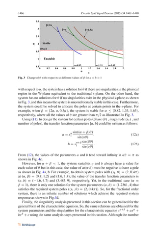
3. Circuits Syst Signal Process (2015) 34:1461–1480 1463
Fig. 1 Stability contour for different values of α
eral fractional order linear time invariant (FLTI) system can be given by (2) for
αi = ki /v.
D(s) = amsαm + · · · + a1sα1 + a0sα0 =
m
i=0
ai s
ki
v , (2)
where ki and v are constant integers. By using the technique in [6,7,35], the charac-
teristic equation of (2) can be written in the W-plane(W = s1/v) as follows:
D(W) = am Wkm + · · · + a1Wk1 + a0Wk0 =
m
i=0
ai Wki , (3)
which is a polynomial in W, then the roots of this equation can be easily obtained
based on the coefficients ai and the powers ki . Generally, these m roots are distributed
in the W-plane; however, the conventional s-plane which is based on the principal
sheet of the Riemann surface and defined by −π s π where its corresponding
region in the W-domain is defined by −π/v W π/v. Moreover, the W-plane
region corresponding to the right half s-plane is defined by−π/2v W π/2v
which reflect the unstable physical poles [35]. The Remaining W-plan which is defined
by| W| π/v is not physical which means that any pole in that region will not have a
corresponding physical pole in the conventional s-plane. Therefore, the corresponding
physical s-plane is mapped into a section in the W-plane, and this section based on the
value of v as shown from Fig.1 where two different contours are depicted at v = 3 and
v = 10. The white and red sections represent the unstable and stable physical s-plane,
while the gray section represents the nonphysical or secondary Riemann sheets.
On the other hand, the system is stable in the time domain if it is a bounded
input bounded output (BIBO) system. So, finite time singularities occur when the

4. 1464 Circuits Syst Signal Process (2015) 34:1461–1480
output variable increases toward infinite at a finite time at certain input in the time
domain [2,6]. Just as the exponential naturally arises out of the solution to integer
order differential equations, the Mittag-Leffler function plays an analogous role in
the solution of non-integer order differential equations [16]. In fact, the exponential
function itself is a very specific form, one of an infinite set, of this seemingly ubiquitous
function. The standard definition of the Mittag-Leffler is given by
Eα,β(z) =
∞
k=0
zk
(αk + β)
, α 0, β 0. (4)
This generalized function will tend to the exponential function as α = β = 1. By
applying the partial fractional concept on the transfer function in (1) and using the
inverse laplace transform using the fact that L(tβ−1 Eα,β(λtα)) = sα−β
(sα−λ) , the time
domain responses can be obtained. The asymptotic behavior of Mittag-Leffler func-
tions plays a very important role in the interpretation of the solution of various prob-
lem. The asymptotic expansion of Eα,β(z) is based on the integral representation of
the Mittag-Leffler function in the form:
Eα,β(z) =
1
2πi
tα−βexp(t)
tα − z
dt, (α) 0, (β) 0, z, α, β ∈ C, (5)
where the path of integration Ω is a loop starting and ending at −∞ and encircling
the circular disk |t| ≤ |z|1/α in the positive sense, |argt| π on Ω. The integral
representation (5) can be used to obtain the asymptotic expansion of the Mittag-Leffler
function at infinity [4,25]. In case of the systems with two fractional order elements,
the value of α is limited as 0 ≤ α ≤ 2. Accordingly, the Mittag-Leffler function has
asymptotic estimates, for example, when 0 α 2 and μ is a real number where
απ
2 μ min[π, απ], then there holds the following asymptotic expansion [16]:
Eα,β(z) =
1
α
z
1−β
α exp(z1/α
) −
N∗
r=1
1
(β − αr)
1
zr
+ O
1
zN∗+1
(6)
as |z| → ∞, |argz| ≤ μ and
Eα,β(z) = −
N∗
r=1
1
(β − αr)
1
zr
+ O
1
zN∗+1
, (7)
as |z| → ∞, μ ≤ |argz| ≤ π
3 System Singularities
The transfer function of the fractional order system with two different fractional order
elements is given by

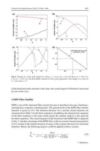
5. Circuits Syst Signal Process (2015) 34:1461–1480 1465
Fig. 2 Change in the number of system poles with respect to α and β when a a = b = 1, b a = 10, b = 10
T (s) =
N(s)
sα+β + asα + b
. (8)
Generally, the system singularities are represented by the denominator and control the
system stability. Hence, the singularities of (8) are obtained by solving the following
polynomial:
sα+β
+ asα
+ b = 0. (9)
To calculate the roots of the polynomial of (9), let s = σ ± jω = s1e± jθ . Therefore,
the polynomial of (9) could be rewritten as follows:
s
α+β
1 ej(α+β)θ
+ asα
1 ejαθ
+ b = 0. (10)
For the traditional systems (α = β = 1), there are always two poles. Yet, for the
fractional orders system, the number of singularities depends on the fractional orders
(α, β) and the transfer function parameters {a, b} as shown in Fig. 2a, b for the two
different cases of (a, b) = (1, 1) and (10, 10), respectively. In addition, the fractional
order system singularities discussed here belong to the essential-type singularities
[10,14]. There are three cases for the number of physical poles in the s-plane of the
fractional order system as follows: no poles in the physical s-plane, two, and four
poles in the physical s-plane as shown in Fig. 2. Thus, the fractional order system
singularities are function of {α + β, α, a, b}. This means, the system can be designed
for a specified singularities, although the number of the fractional order elements is
constant which adds more design degree of freedom to the system design.
By equating the real and imaginary parts of (10) to zero and using simple trigono-
metric relations, the poles of the system are given by
s1 =
−a sin(αθ)
sin((α + β)θ)
1/β
=
−b sin((α + β)θ)
a sin(βθ)
1/α
. (11)
From (11), the value of θ is a function of the fractional orders (α, β) and the parameters
(a, b) thus increasing the design degree of freedom. By solving (11) numerically for θ

6. 1466 Circuits Syst Signal Process (2015) 34:1461–1480
Fig. 3 Change of θ with respect to α different values of β for a = b = 1
with respect to α, the system has a solution for θ if there are singularities in the physical
region in the W-plane equivalent to the traditional s-plane. On the other hand, the
system has no solutions for θ if no singularities exist in the physical s-plane as shown
in Fig. 3, and this means the system is unconditionally stable in this case. Furthermore,
the system could be solved to allocate the poles at certain points in the s-plane. For
example, when β = {2α, α, 0.5α}, the system is stable for α ≤ {0.82, 1.33, 1.63},
respectively, where all the values of θ are greater than π/2 as illustrated in Fig. 3.
Using (11), to design the system for certain poles (phase (θ) , magnitude (s1) , and
number of poles), the transfer function parameters {a, b} could be written as follows:
a = sα
1
sin((α + β)θ)
sin(αθ)
, (12a)
b = s
α+β
1
sin(βθ)
sin(αθ)
. (12b)
From (12), the values of the parameters a and b tend toward infinity at αθ = π as
shown in Fig. 4c.
However, for α + β 1, the system variables a and b always have a value for
each value of θ but in this case, the value of a(or b) must be negative to have a pole
as shown in Fig. 4a, b. For example, to obtain system poles with (s1, θ) = (2, 0.4π)
at (α, β) = (0.8, 1.2) and (1.6, 1.8), the value of the transfer function parameters is
(a, b) = (−1.6, 4.7) and (3.485, 9), respectively. Yet, in the traditional case (α =
β = 1), there is only one solution for the system parameters (a, b) = (1.2361, 4) that
satisfies the required system poles ((s1, θ) = (2, 0.4π)). So, for the fractional order
system, there is an infinite number of solutions which achieve the required system
response as shown in Fig.4d.
Finally, the singularity analysis presented in this section can be generalized for the
general form of the characteristic equation. So, the same relations are obtained for the
system parameters and the singularities for the characteristic equation sα+β + asα +
bsβ + c using the same analysis steps presented in this section. Although the number

7. Circuits Syst Signal Process (2015) 34:1461–1480 1467
0.5 1 1.5 2 2.5 3
-4
-3
-2
-1
0
1
2
3
θ
System
Variables
(a,b)
a
b
(a)
α
β
0.5 1 1.5
0.5
1
1.5
2
Valid solution for the system
parameters a and b
(d)
(c)
(b)
Fig. 4 Change of a and b with respect to θ when s1 = 2 a (α, β) = (0.3, 0.5) b (α, β) = (0.8, 1.2),
c (α, β) = (1.6, 1.8), and d Available solutions for the system parameters with change in α and β at
θ = 0.4π and s1 = 2
of the fractional order elements is the same, the system degree of freedom is increased
by one in this case.
4 KHN Filter Stability
KHN is one of the important filter circuits because it introduces low-pass, band-pass,
and high-pass responses simultaneously. The general form of the KHN filter transfer
function is given in (13). The relations between N(s) and the circuit elements are
summarized in Table 1 for the three responses. In addition, the characteristic equation
of the three responses is the same which means the stability analysis is the same for
the three responses. The circuit diagram of the fractional order KHN filter is depicted
in Fig. 5. Another advantage of the KHN filter is that its transfer function presented in
(13) is similar to the transfer function of many of the systems that have two fractional
elements. Hence, the following analysis could be applied to these systems.
V1
Vin
=
N(s)
sα+β + R3
R1C1
(R5/R6)
R3+R4
sα + R5/R6
C1C2 R1 R2
. (13)

8. 1468 Circuits Syst Signal Process (2015) 34:1461–1480
Table 1 Summary of the relations between the circuit elements and the transfer function parameters
Parameter Relation
FLPF FBPF FHPF
N(s)
R5/R6
C1C2 R1 R2
R4
R3+R4
sα 1
C1 R1
R5/R6
C1C2 R1 R2
R4
R3+R4
sα+β R5/R6
C1C2 R1 R2
R4
R3+R4
a
R3
R1C1
(R5/R6)
R3+R4
R3
R1C1
(R5/R6)
R3+R4
R3
R1C1
(R5/R6)
R3+R4
b
R5/R6
C1C2 R1 R2
R5/R6
C1C2 R1 R2
R5/R6
C1C2 R1 R2
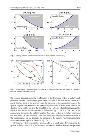
Fig. 5 Fractional order KHN filter
Although the design and analysis of the fractional order KHN filter have been presented
before [1,12,42,43], the stability analysis of these filters was not presented. So, this
section focuses on the stability analysis of the KHN filters. As the transfer function of
(13) is the same as the transfer function of (8), the equation of (8) will be used in the
following analysis, and then the relations tabulated in Table 1 are used to calculate the
circuit elements value. So, the condition of stability for the traditional fractional order
system is obtained by substituting θ = π/2 in (11) which represents the boundary line
s = ± jω as follows.
−a sin(0.5απ)
sin(0.5(α + β)π)
α
=
−b sin(0.5(α + β)π)
a sin(0.5βπ)
β
, α + β = 2, (14a)
ωo =
−a sin(0.5απ)
sin(0.5(α + β)π)
1/β
=
−b sin(0.5(α + β)π)
a sin(0.5βπ)
1/α
, α + β = 2. (14b)
Consequently, the system stability is dependent on the parameters{α, β, a, b} which
means extra degree of freedom. So, the stability condition of (14a) can be used to draw
a stability contour for the filter at different combinations of the equation parameters.
From (14b), for ωo to be real positive at α + β 2, the value of a must be positive
(a 0) and b/a 0. On the contrary, when α + β 2, it should be a 0 and
b/a 0 for the value of ωo to be a real positive value as shown in Fig. 6. In addition,
for α + β 1, the value of b must be positive for the system to be stable. On the
other hand, the stability contours in the α − β plane using (14) are illustrated in Fig.
7 at different values of the transfer function parameters a and b. The region under

9. Circuits Syst Signal Process (2015) 34:1461–1480 1469
Fig. 6 Stability contours for the transfer function of (8) at different values of (α, β)
0.2 0.4 0.6 0.8 1 1.2 1.4 1.6 1.8
0
0.5
1
1.5
2
(a) (b)
α
β
a=-1
a=3
a=1
a=0.01
0 0.5 1 1.5 2
0
0.5
1
1.5
2
α
β
b=2
b=6
b=0.1
Fig. 7 System stability contour in the α − β plane, a for different values of a and when b = 1, and b for
different values of b and when a = 1
the contour line represents the combination of the fractional orders α and β which
produces a stable system at the given value of a and b. Indeed, as the values of α
and β become close to the contour lines, the damping in the system increases as the
system singularities become closer to the imaginary axis. When a tends to zero, the
stability curve will be close to the straight line (α + β = 2) where the area under this
line is stable and above it is unstable as depicted in Fig. 7a for a = 0.01. Yet, as the
parameter a increases, the stability contour line starts to take a curvature shape and
the area under the line increases. Then, the stable area increases with the increase in
the parameters a. On the contrary, the increase in the transfer function parameter b
reduces the stable region as shown in Fig. 7b.
Obviously, system singularities are considered a vital factor for measuring the
system stability. Hence, it is necessary to present the relation between the previous

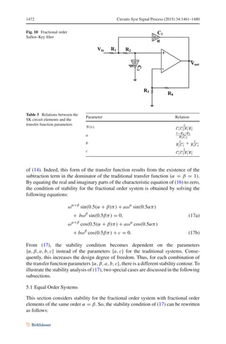
10. 1470 Circuits Syst Signal Process (2015) 34:1461–1480
Fig. 8 Movement of the system singularities with respect to a and b, a for b = 1, α = 1.2, and β = 0.6,
b for b = 1, α = 1.6, and β = 1.8, c for a = 1, α = 1.2, and β = 0.6, and d for a = 1, α = 1.6, and
β = 1.8
analysis and the system singularities to verify the analysis. Consequently, the study of
the system singularity movement due to the transfer function parameters {a, b, α, β}
is illustrated in Fig. 8. For small values of a, the system starts unstable and then the
singularities move toward the stable region as the value of the parameter a increases
as shown in Fig. 8a, b. This is the same result obtained before from the stability
contours of Fig. 7a. On the other hand, the system is unstable for b 0 as mentioned
before in Fig 6. Yet, for b ≥ 0, the system starts stable and moves toward the unstable
region as b increases as depicted in Fig. 8c, d. Accordingly, the singularities movement
due to the system parameters matches with the proposed stability contour analysis.
Then, these stability contours provide an easy and fast way to determine the system
stability. In addition, the number of poles is also dependent on the parameters a and
b as summarized in Table 2 which confirms the results discussed before.
The frequency response of the KHN filter using ADS is presented in Fig. 9 at
different fractional orders for a = b = 1. As the point (α, β) = (1.2, 1.5) is very
close to the stability contour (from Fig 7a), the damping in the filter response is very
large as expected. On the other hand, the points (α, β) = (0.7, 0.7) and (0.8, 1.3) are
far from the stability contour and this makes their frequency response to have a very
small damping as depicted in Fig. 9.
5 Sallen–Key Filter Stability
Sallen–Key (SK) filters are considered one of the most common and well-known filter
family [37,38]. The conventional Sallen–Key family provides a second order filters by
using two integer order capacitors and one op-amp. Although the design and analysis

11. Circuits Syst Signal Process (2015) 34:1461–1480 1471
Table 2 Summary of the stability analysis in the s-plane
(α, β) a b Number of poles Stable/unstable
(1.2, 0.6) −20 ≤ a −0.3 1 2 Unstable
a ≥ −0.3 1 2 Stable
(1.6, 1.8) −20 ≤ a ≤ −1.3 1 2 Unstable
−1.3 a ≤ 1.9 1 4 Unstable
a 1.9 1 4 Stable
(1.2, 0.6) 1 b 0 1 Unstable
1 b ≥ 0 2 stable
(1.6, 1.8) 1 b 0 3 Unstable
1 0 ≥ b ≤ 0.2 4 Stable
1 b 0.2 4 Unstable
Fig. 9 KHN frequency
response at a = b = 1
of the fractional order Sallen–Key filter were introduced before in [41], the stability
analysis was not discussed in detail. Therefore, this work studies the Sallen–Key filter
stability using two different fractional order elements of different orders (α, β). The
transfer function of the fractional order Sallen–Key filter illustrated in Fig. 10 is given
as follows:
Vout
Vin
=
1
C1C2 R1 R2
sα+β + 1−R4/R3
R2C2
sα +
1
R2C1
+ 1
R1C1
sβ + 1
C1C2 R1 R2
. (15)
To simplify the analysis, the transfer function of (15) can be rewritten as follows:
T (s) =
N(s)
sα+β + asα + bsβ + c
, (16)
where a, b, andc are constants and α and β are the fractional orders and 0 α, β ≤ 2.
The relation between the transfer function parameters and the circuit elements is
summarized in Table 3. Basically, the transfer function of (16) is the general form
of the transfer function of fractional order system with two different fractional order
elements. So, for the special case of a = 0 or b = 0, the transfer function of (16)
returns to the form of (8) and hence the filter stability is controlled by the relation

12. 1472 Circuits Syst Signal Process (2015) 34:1461–1480
Fig. 10 Fractional order
Sallen–Key filter
Table 3 Relations between the
SK circuit elements and the
transfer function parameters
Parameter Relation
N(s) 1
C1C2 R1 R2
a
1−R4/R3
R2C2
b 1
R2C1
+ 1
R1C1
c 1
C1C2 R1 R2
of (14). Indeed, this form of the transfer function results from the existence of the
subtraction term in the dominator of the traditional transfer function (α = β = 1).
By equating the real and imaginary parts of the characteristic equation of (16) to zero,
the condition of stability for the fractional order system is obtained by solving the
following equations:
ωα+β
sin(0.5(α + β)π) + aωα
sin(0.5απ)
+ bωβ
sin(0.5βπ) = 0, (17a)
ωα+β
cos(0.5(α + β)π) + aωα
cos(0.5απ)
+ bωβ
cos(0.5βπ) + c = 0. (17b)
From (17), the stability condition becomes dependent on the parameters
{α, β, a, b, c} instead of the parameters {a, c} for the traditional systems. Conse-
quently, this increases the design degree of freedom. Thus, for each combination of
the transfer function parameters {α, β, a, b, c}, there is a different stability contour. To
illustrate the stability analysis of (17), two special cases are discussed in the following
subsections.
5.1 Equal Order Systems
This section considers stability for the fractional order system with fractional order
elements of the same order α = β. So, the stability condition of (17) can be rewritten
as follows:

13. Circuits Syst Signal Process (2015) 34:1461–1480 1473
Fig. 11 Stability contour of the
fractional order system at
different values of c
0 0.2 0.4 0.6 0.8 1 1.2 1.4 1.6 1.8 2
-15
-10
-5
0
5
10
15
α
X
c=20
c=10
c=40
Unstable region
Stable region
ω2α
cos(απ) + (a + b)ωα
cos(0.5απ) + c = 0, (18a)
ωα
sin(απ) + (a + b) sin(0.5απ) = 0. (18b)
Then, for X = a + b and making some simplifications, the stability condition for this
case can be determined by
X = ±2
c cos(0.5απ). (19)
For the value of X to be a real value, the value of c must be greater than zero which
means the system cannot be designed for c 0 in this case. The stability contour of
the fractional order system in this case is illustrated in Fig. 11 for different values of
c. The interesting result here is that the parameter X takes positive or negative values
and the system remains in the stable region, which means the system can be designed
for negative values of X. This increases the design flexibility.
5.2 Fractional Order System of Dependent Orders
In the following analysis of the fractional order system stability, the fractional orders α
and β are dependent by a factor k where 0 α, kα ≤ 2. Then, under these conditions,
the transfer function of (16) can be written as follows:
T (s) =
N(s)
sα(1+k) + asα + bskα + c
. (20)
By equating the real and imaginary parts of the characteristic equation of (20), the
stability condition can be calculated from the following relations.
ωα(1+k)
cos(0.5α(1 + k)π) + aωα
cos(0.5απ)+
bωαk
cos(0.5αkπ) + c = 0, (21a)
ωα(1+k)
sin(0.5α(1 + k)π) + aωα
sin(0.5απ)+
bωαk
sin(0.5αkπ) = 0. (21b)

14. 1474 Circuits Syst Signal Process (2015) 34:1461–1480
By solving (21a, b) together, the stability contour for the transfer function of (20) is
obtained. To demonstrate the effect of the transfer function parameters on the system
stability, a special case for k = 2 is studied in the following analysis. So for k = 2,
the oscillation frequency and the condition of oscillation are given by
ωosc =
cos(0.5απ)
4(cos(0.5απ))2 − 1
− b ±
(b2 − a(4 − (sec(0.5απ))2))
1/α
, (22a)
ω3α
osc cos(1.5απ) + bω2α
osc cos(απ) + aωα
osc cos(0.5απ) + c = 0. (22b)
From (22a), the frequency of oscillation ωosc is a function of the parameters {a, b, α}
which increases the degree of freedom. In addition, the oscillation frequency ωosc is
independentonthevalueofc,andthisgreatadvantagecanbeusedtomakeindependent
control on the condition of stability and the oscillation frequency. As shown in Fig.
12, the system of (22) has three regions for the oscillation frequency depending on the
value a, b, and α. These three regions are as follows: no solution for ωosc, one solution
exists for ωosc, and finally two solutions for ωosc exist. Furthermore, the separation
between any two regions with the change in the fractional order α occurs always at the
same value of α which is called αc, and from (22a), this value equals 2/3. The stability
contours are also illustrated in Fig. 12 versus the parameters c for the same cases of the
parameters a and b. Actually, for α αc, the filter becomes more stable as the value
of c increases. On the contrary, for α αc, the system moves toward the unstable
region as the value of c increases. Although there are two solutions for the oscillation
frequency at some cases ((a, b) = (5, −5)), there is only one stability contour because
one of these values corresponds to a negative value of the parameters c. Thus, the filter
in this case is unreliable which means this second contour line is ignored like the
dashed line of the stability contour of (a, b) = (5, −5) of Fig. 12. A summary of the
relations between the oscillation frequency and the system parameters a, b, and α is
shown in Fig. 13. Moreover, the parameter a has a similar effect on the oscillation
frequency. Hence, there is a critical value of a which represents the border line between
the two regions mentioned before for the oscillation frequency (no solution and two
solutions exist), and this value of a is defined as ac. Then from (22a), the value of ac
is defined as follows:
ac =
b2
4 − (sec(0.5απ))2
. (23)
Traditionally, poles are used to determine the system stability. Consequently, it is nec-
essary to prove the proposed analysis by comparing it with the singularities movement
of the system. For fixed values of the fractional order α and the parameters b and c,
as the value of a increases the system singularities move toward the stable region and
the system becomes more stable as shown in Fig. 14a. Due to the symmetry of the
transfer function, the effect of the parameter b on the system singularities and hence
the stability is similar to the effect of a as depicted in Fig. 14b. On the other hand, as the
value of c increases, the system singularities move toward the unstable region as shown

15. Circuits Syst Signal Process (2015) 34:1461–1480 1475
Fig. 12 Change in the oscillation frequency (ωα
osc) and the stability contour with α at different values of
a and b
Fig. 13 Summary of the effect of a and α on the oscillation frequency ωosc

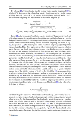
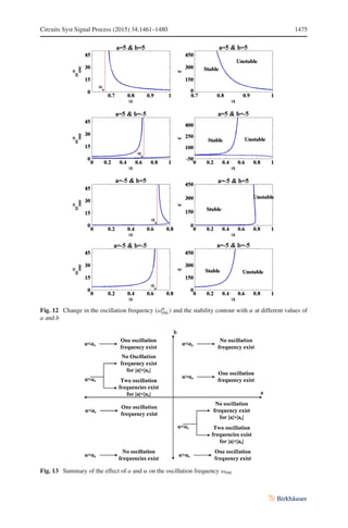
16. 1476 Circuits Syst Signal Process (2015) 34:1461–1480
Fig. 14 Singularities movement with respect to a, b, and c for α = 0.8, a b = 1 and c = 1, b a = 1 and
c = 1, and c a = b = 1
Fig. 15 Numerical simulation for the fractional order filter at different cases of the fractional orders
in Fig. 14c because α αc as expected before. Then, the poles movement transfer
function parameters matches with previous analysis. Finally, the work presented in
this subsection can be generalized for any value of k.
Using the proposed stability analysis and the fractional order SK filter design
method proposed in [41], numerical and experimental work for fractional order SK
filter is presented to prove the reliability of the proposed analysis. For equal orders
(α = β = 1.2) and for c = 10, then from Fig. 11 for the filter to be stable the value
of X −1.9. The numerical analysis for the cases of (α, X) = (1.2, −1.8), (1.2, 5)
is depicted in Fig. 15. The damping for the case of X = −1.8 is greater than the

17. Circuits Syst Signal Process (2015) 34:1461–1480 1477
Fig. 16 a Equivalent RC tree circuit of the fractional order element of any order[18], and b The GIC circuit
used to simulate fractional order element with order greater than unity [5]
case of the case of X = 5 because in the first case, the value of X is very close to
the stability contour. Thus, for the filter to be stable without damping, the value of
X should be far away from the stability contour as mentioned before. On the other
hand, two SK filters of dependent orders with k = 2 are illustrated in Fig. 15 with the
orders (α, β) = (0.6, 1.2) and (a, b) = (−5, 5). In this case, for the filter to be stable
and from Fig. 12, the value of c 4. As shown in Fig. 15, the damping for the case
of c = 4.5 is greater than the damping in the case of c = 50 because as expected.
Finally, the relations tabulated in Table 3 are used to obtain the circuit components
values. To study the fractional order filter experimentally, an equivalent RC circuit
for the fractional order element of order less than unity based on the finite element
approximation is illustrated in Fig. 16a [18]. The values of the resistances and capac-
itors of the equivalent circuit composed of fractional order capacitor with YF = sαCF
are given by the following relations [18]:
Rfn =
YF (α) sin(απ)
π
σα
n

18. (ln(σ))
−1
, (24a)
Cfn =
YF (α) sin(απ)
π
σα−1
n

19. (ln(σ)), (24b)

20. 1478 Circuits Syst Signal Process (2015) 34:1461–1480
Fig. 17 a Photo of the practical fractional Sallen–Key filter. b Experimental results of the fractional Sallen–
Key filter
where YF is the admittance value, σ is the relaxation rate corresponding to the pole of
the nth branch, and