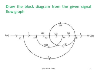
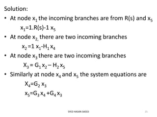
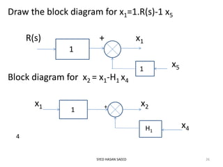
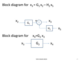
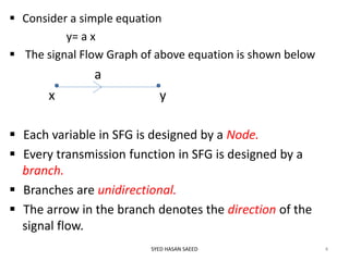
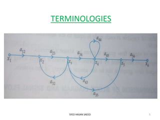
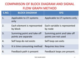
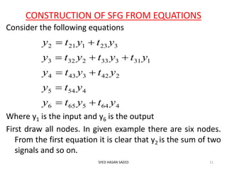
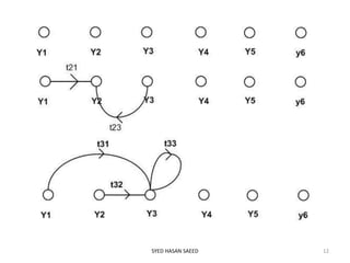
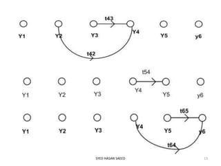
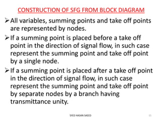
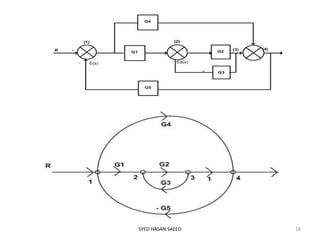
This document provides an overview of signal flow graphs (SFG). It defines SFG as a graphical representation of linear systems, where each variable is represented by a node and transmissions are branches with arrows denoting signal flow direction. Key terms are defined, including input/output nodes, mixed nodes, transmittance, forward paths, loops, and path/loop gains. Properties and examples of SFG construction from equations and block diagrams are described. Mason's gain formula is introduced for determining overall transfer functions from SFGs. The effects of feedback on gain and stability are also briefly discussed.

1. SIGNAL FLOW GRAPH
(SFG)
SYED HASAN SAEED 1

2. OUTLINE
Introduction to signal flow graph.
 Definitions
 Terminologies
 Properties
 Examples
Mason’s Gain Formula.
Construction of Signal Flow Graph.
Signal Flow Graph from Block Diagram.
Block Diagram from Signal Flow Graph.
Effect of Feedback.
SYED HASAN SAEED 2

3. INTRODUCTION
• SFG is a simple method, developed by S.J.Mason
• Signal Flow Graph (SFG) is applicable to the linear
systems.
• It is a graphical representation.
• A signal can be transmitted through a branch only
in the direction of the arrow.
SYED HASAN SAEED 3

4.  Consider a simple equation
y= a x
 The signal Flow Graph of above equation is shown below
a
x y
 Each variable in SFG is designed by a Node.
 Every transmission function in SFG is designed by a
branch.
 Branches are unidirectional.
 The arrow in the branch denotes the direction of the
signal flow.
SYED HASAN SAEED 4

5. TERMINOLOGIES
SYED HASAN SAEED 5

6. Input Node or source node: input node is a node
which has only outgoing branches. X1 is the input
node.
Output node or sink node: an output node is a node
that has only one or more incoming branches. X6 is
the output node.
Mixed nodes: a node having incoming and outgoing
branches is known as mixed nodes. x2, x3, x4 and x5
are the mixed nodes.
Transmittance: Transmittance also known as transfer
function, which is normally written on the branch
near arrow.
SYED HASAN SAEED 6

7. Forward path: Forward path is a path which
originates from the input node and terminates at the
output node and along which no node is traversed
more than once. X1-x2-x3-x4-x5-x6 and x1-x2-x3-x5-x6 are
forward paths.
Loop: loop is a path that originates and terminates on
the same node and along which no other node is
traversed more than once. e.g x2 to x3 to x2 and x3 to
x4 to x3 .
Self loop: it is a path which originates and terminates
on the same node. For example x4
SYED HASAN SAEED 7

8. SYED HASAN SAEED 8
Path gain: The product of the branch gains along
the path is called path gain. For example the gain
of the path x1-x2-x3-x4-x5-x6 is a12a23a34a45a56
 Loop Gain: The gain of the loop is known as loop
gain.
Non-touching loop: Non-touching loops having no
common nodes branch and paths. For example x2
to x3 to x2 and x4 to x4 are non-touching loops.

9. PROPERTIES OF SIGNAL FLOW GRAPH:
1. Signal flow graph is applicable only for linear time-
invariant systems.
2. The signal flow graph along the direction of the
arrow.
3. The gain of the SFG is given by Mason’s formula.
4. The signal gets multiplied by branch gain when it
travels along it.
5. The SFG is not be the unique property of the sytem.
6. Signal travel along the branches only in the direction
described by the arrows of the branches.
SYED HASAN SAEED 9

10. COMPARISON OF BLOCK DIAGRAM AND SIGNAL
FLOW GRAPH METHOD
S.NO. BLOCK DIAGRAM SFG
1. Applicable to LTI systems
only
Applicable to LTI systems only
2. Each element is represented
by block
Each variable is represented
by node
3. Summing point and take off
points are separate
Summing point and take off
points are not used
4. Self loop do not exists Self loop can exits
5. It is time consuming method Requires less time
6. Feedback path is present Feedback loops are present.
SYED HASAN SAEED 10

11. CONSTRUCTION OF SFG FROM EQUATIONS
Consider the following equations
Where y1 is the input and y6 is the output
First draw all nodes. In given example there are six nodes.
From the first equation it is clear that y2 is the sum of two
signals and so on.
SYED HASAN SAEED 11
4645656
4545
2423434
1313332323
3231212
ytyty
yty
ytyty
ytytyty
ytyty






12. SYED HASAN SAEED 12

13. SYED HASAN SAEED 13

14. Complete Signal Flow Graph
SYED HASAN SAEED 14

15. CONSTRUCTION OF SFG FROM BLOCK DIAGRAM
All variables, summing points and take off points
are represented by nodes.
If a summing point is placed before a take off
point in the direction of signal flow, in such case
represent the summing point and take off point
by a single node.
If a summing point is placed after a take off point
in the direction of signal flow, in such case
represent the summing point and take off point
by separate nodes by a branch having
transmittance unity.
SYED HASAN SAEED 15

16. SYED HASAN SAEED 16

17. Draw the SFG for the network shown in fig, take
V3 as output node
SYED HASAN SAEED 17

18. SYED HASAN SAEED 18
243
2
3
2
2
2
2313213332
1
2
1
1
1
)(
iRv
R
v
R
v
i
iRiRiiRRiv
R
v
R
v
i





19. MASON’S GAIN FORMULA
SYED HASAN SAEED 19
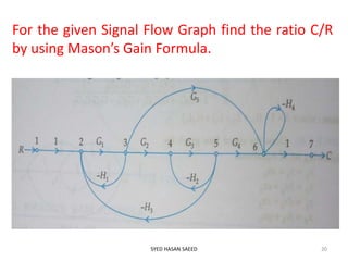
By using Mason’s Gain formula we can determine the
overall transfer function of the system in one step.
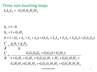
Where Δ=1- [sum of all individual loop gain]+[sum of
all possible gain products of two non-touching
loops]-[sum of all possible gain products of three
non-touching loops]+…………
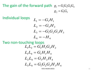
gk = gain of kth forward path
Δk =the part of Δ not touching the kth forward path



 kkg
T

20. For the given Signal Flow Graph find the ratio C/R
by using Mason’s Gain Formula.
SYED HASAN SAEED 20

21. The gain of the forward path
Individual loops
Two non-touching loops
SYED HASAN SAEED 21
512
43211
GGg
GGGGg


44
33213
232
111
HL
HGGGL
HGL
HGL




4332143
42342
41141
231121
HHGGGLL
HHGLL
HHGLL
HGHGLL





22. Three non-touching loops
SYED HASAN SAEED 22
4213143321423411
2131433212311
23514321
2211
421434241214321
232
1
42311421
1
)1(
)()()(1
1
01
HHHGGHHGGGHHGHHG
HHGGHHGGGHGHG
HGGGGGGG
R
C
gg
R
C
LLLLLLLLLLLLLLL
HG
HHGHGLLL












23. BLOCK DIAGRAM FROM SFG
For given SFG, write the system equations.
At each node consider the incoming branches
only.
Add all incoming signals algebraically at a node.
 for + or – sign in system equations use a
summing point.
For the gain of each branch of signal flow graph
draw the block having the same transfer function
as the gain of the branch.
SYED HASAN SAEED 23

24. Draw the block diagram from the given signal
flow graph
SYED HASAN SAEED 24

25. Solution:
• At node x1 the incoming branches are from R(s) and x5
x1=1.R(s)-1 x5
• At node x2, there are two incoming branches
x2 =1 x1-H1 x4
• At node x3 there are two incoming branches
X3 = G1 x2 – H2 x5
• Similarly at node x4 and x5 the system equations are
X4=G2 x3
x5=G3 x4 +G4 x3
SYED HASAN SAEED 25

26. Draw the block diagram for x1=1.R(s)-1 x5
R(s) + x1
x5
Block diagram for x2 = x1-H1 x4
x1 + x2
x4
4
SYED HASAN SAEED 26
1
1
H1
1

27. Block diagram for x3 = G1 x2 – H2 x5
x2 + x3
x5
Block diagram for x4=G2 x3
x3 G2 x4
SYED HASAN SAEED 27
G1
H2

28. Block diagram for x5=G3 x4 +G4 x3
x4 + x5
+
x3
SYED HASAN SAEED 28
G3
G4

29. Combining all block diagram
SYED HASAN SAEED 29

30. EFFECT OF FEEDBACK ON OVERALL GAIN
R(s) C(s)
The overall transfer function of open loop system is
The overall transfer function of closed loop system is
For negative feedback the gain G(s) is reduced by a factor
So due to negative feedback overall gain of the system is
reduced
SYED HASAN SAEED 30
G(s)
)(
)(
)(
sG
sR
sC

)()(1
)(
)(
)(
sHsG
sG
sR
sC


)()(1
1
sHsG

31. EFFECT OF FEEDBACK ON STABILITY
SYED HASAN SAEED 31
Consider the open loop system with overall transfer
function
The pole is located at s=-T
Now, consider closed loop system with unity negative
feedback, then overall transfer function is given by
Now closed loop pole is located at s=-(T+K)
Thus, feedback controls the time response by adjusting the
location of poles. The stability depends upon the location
of the poles. Thus feedback affects the stability.
Ts
K
sG

)(
)()(
)(
KTs
K
sR
sC

