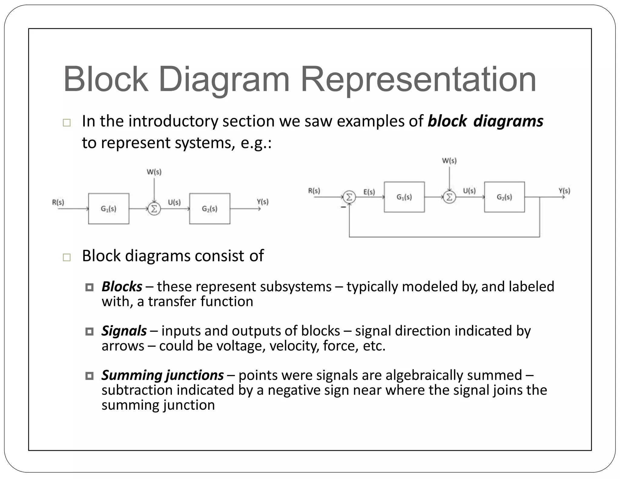
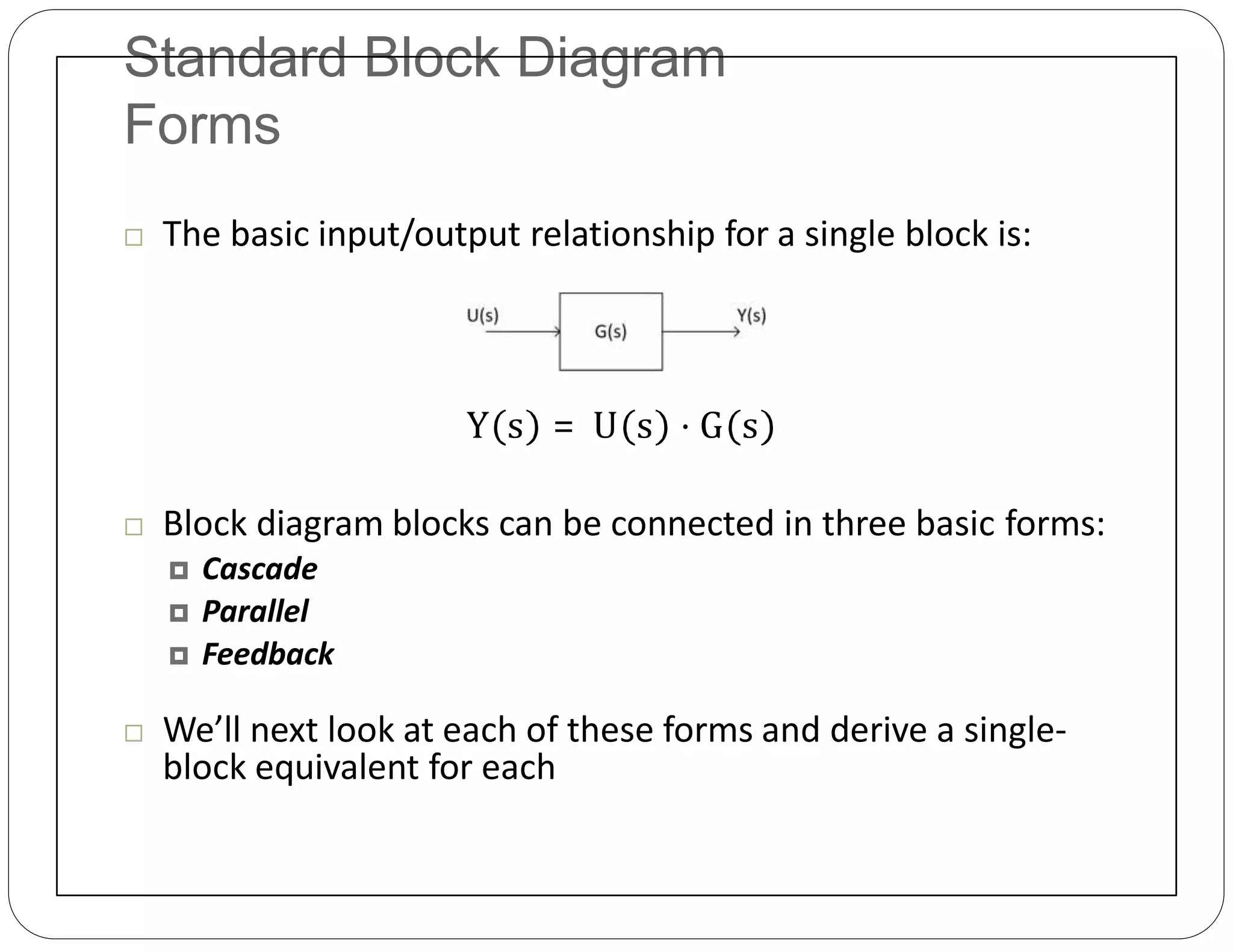
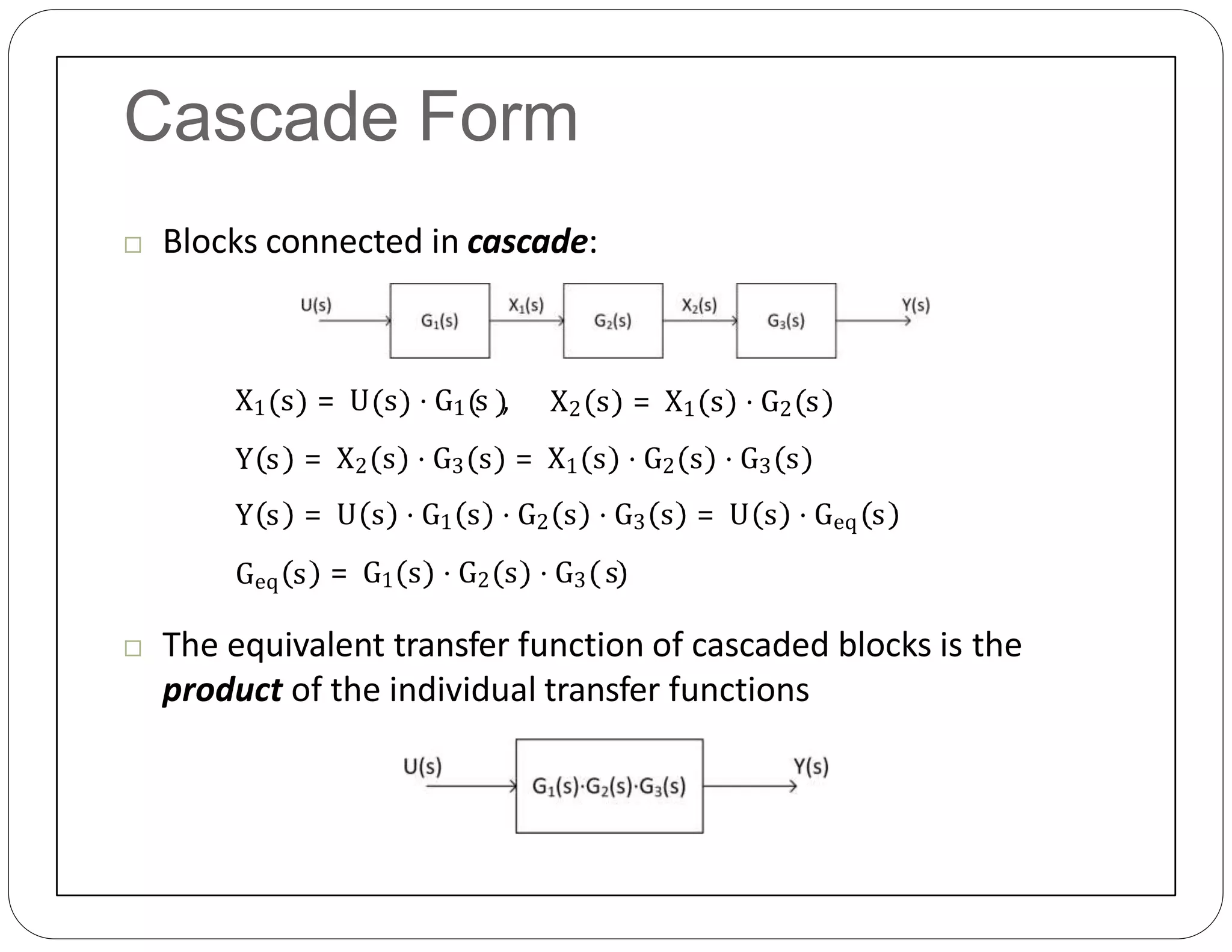
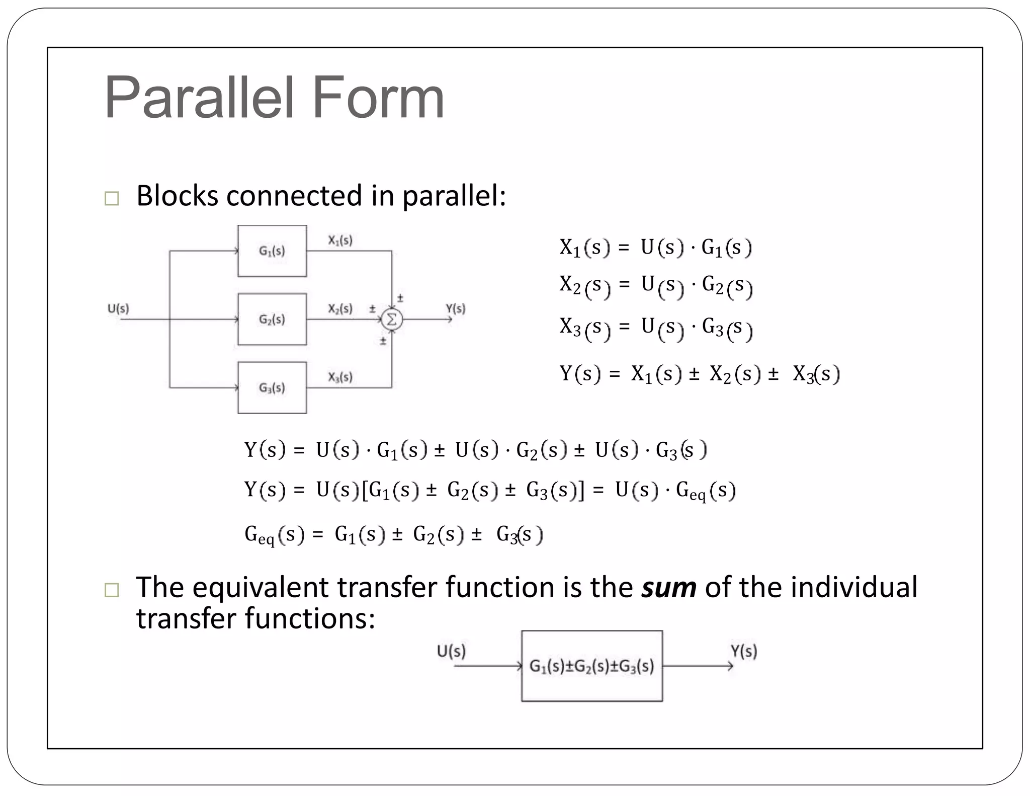
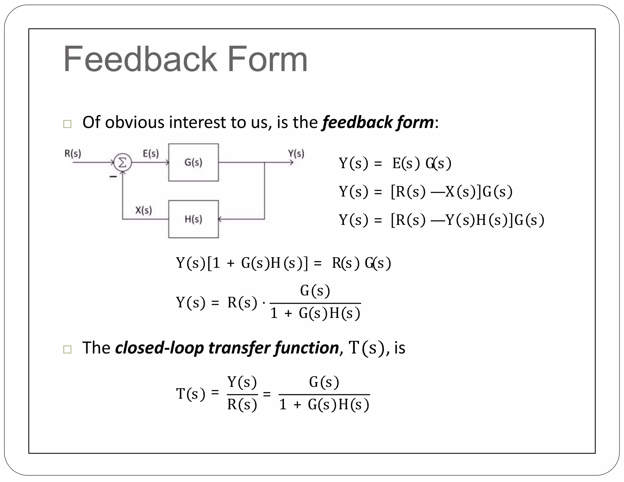
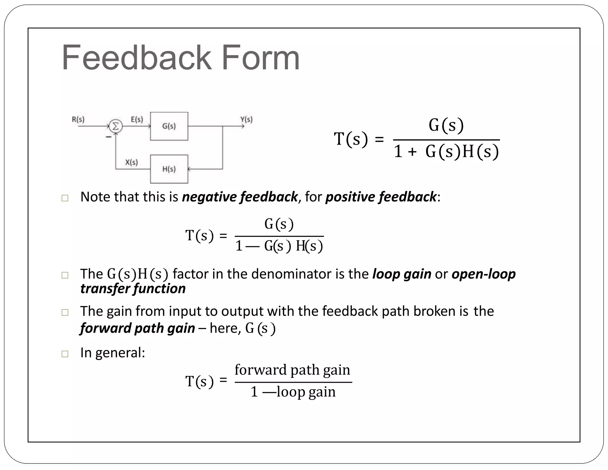
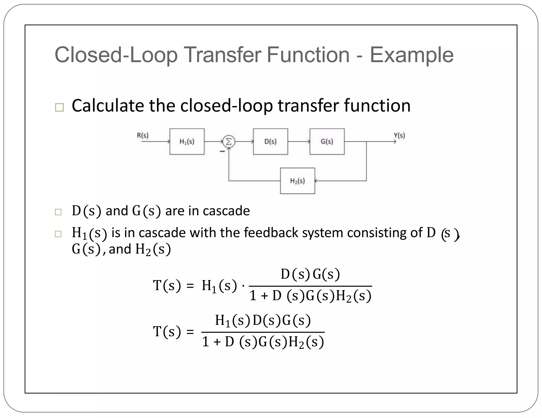
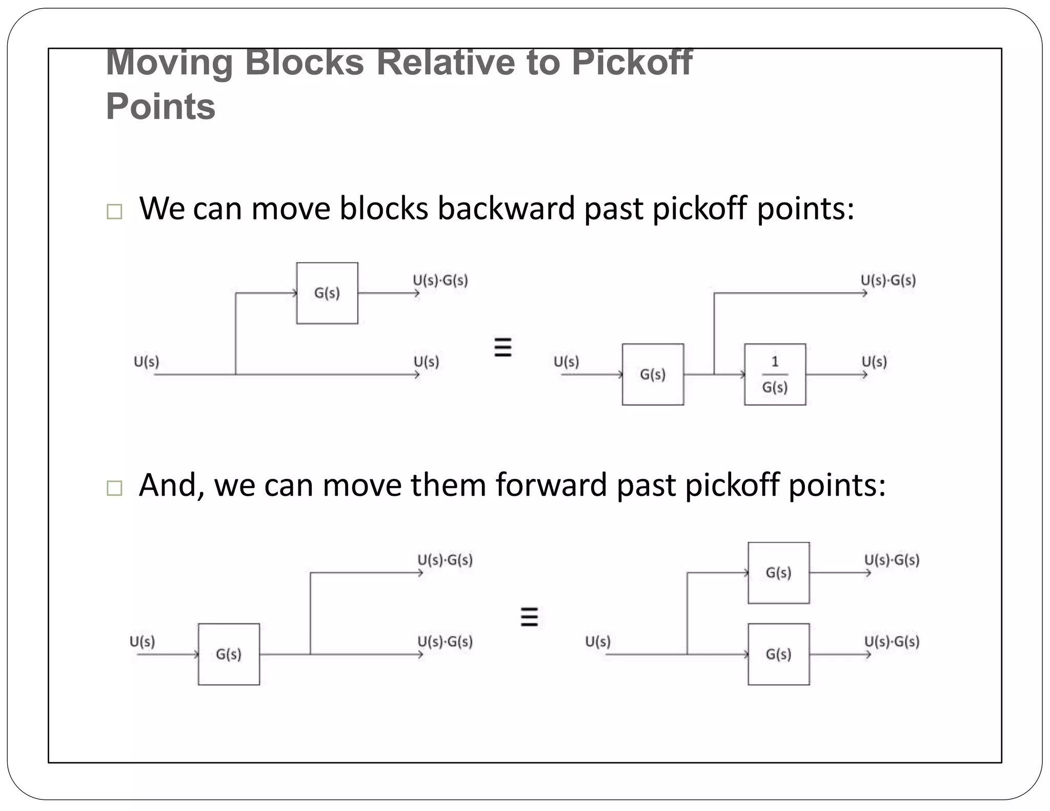
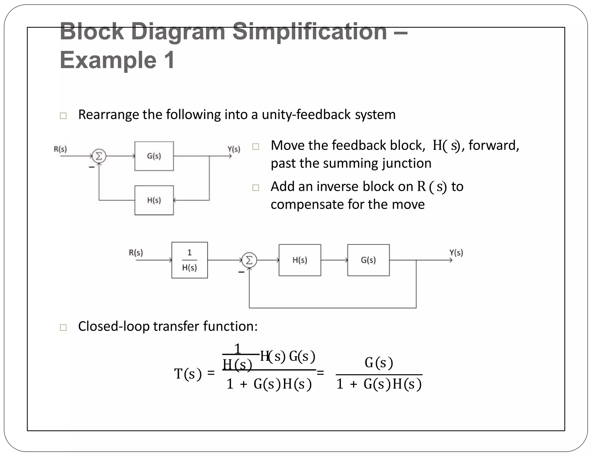
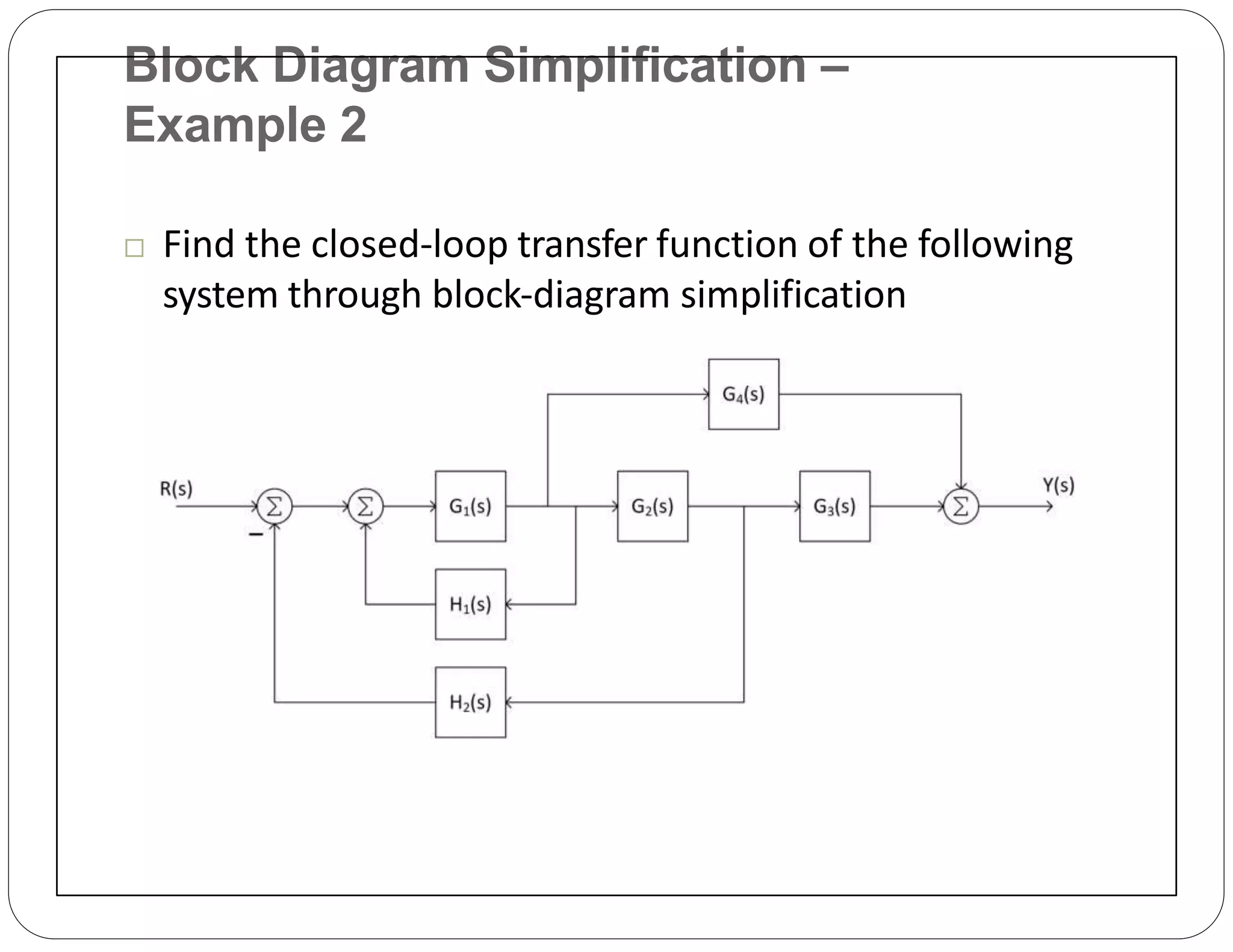
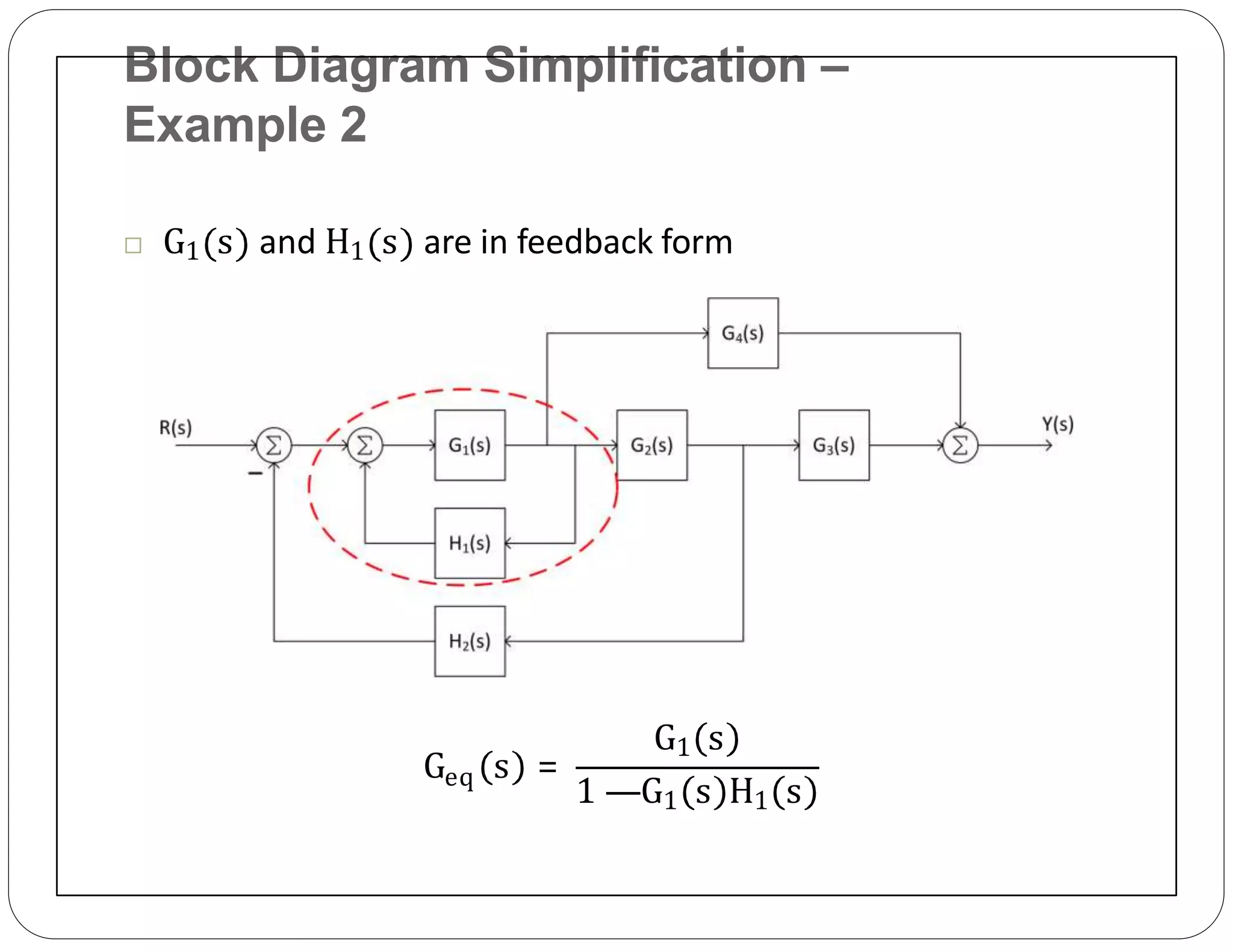
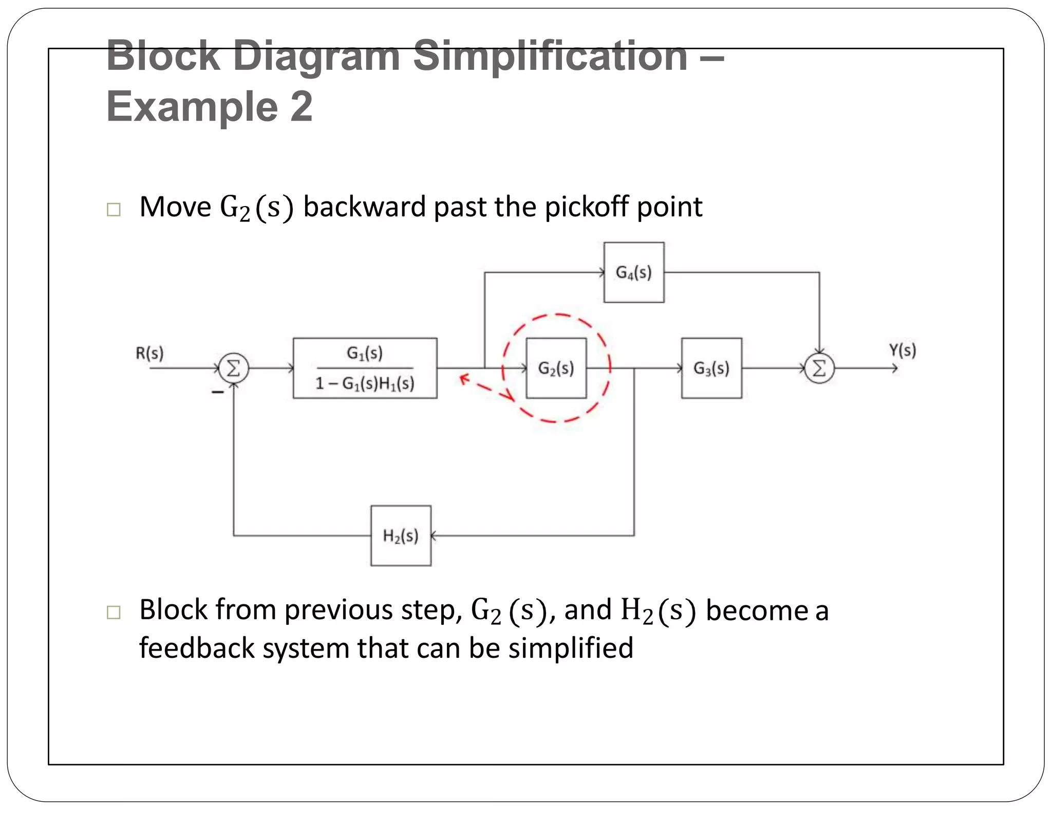
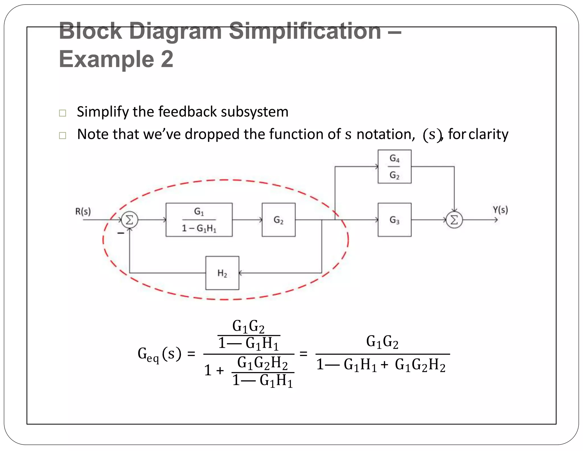
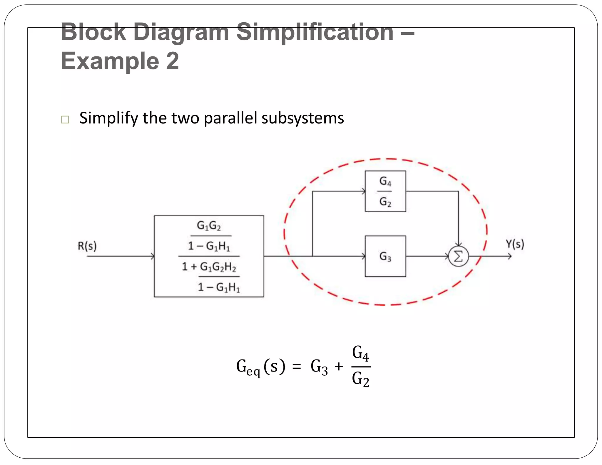
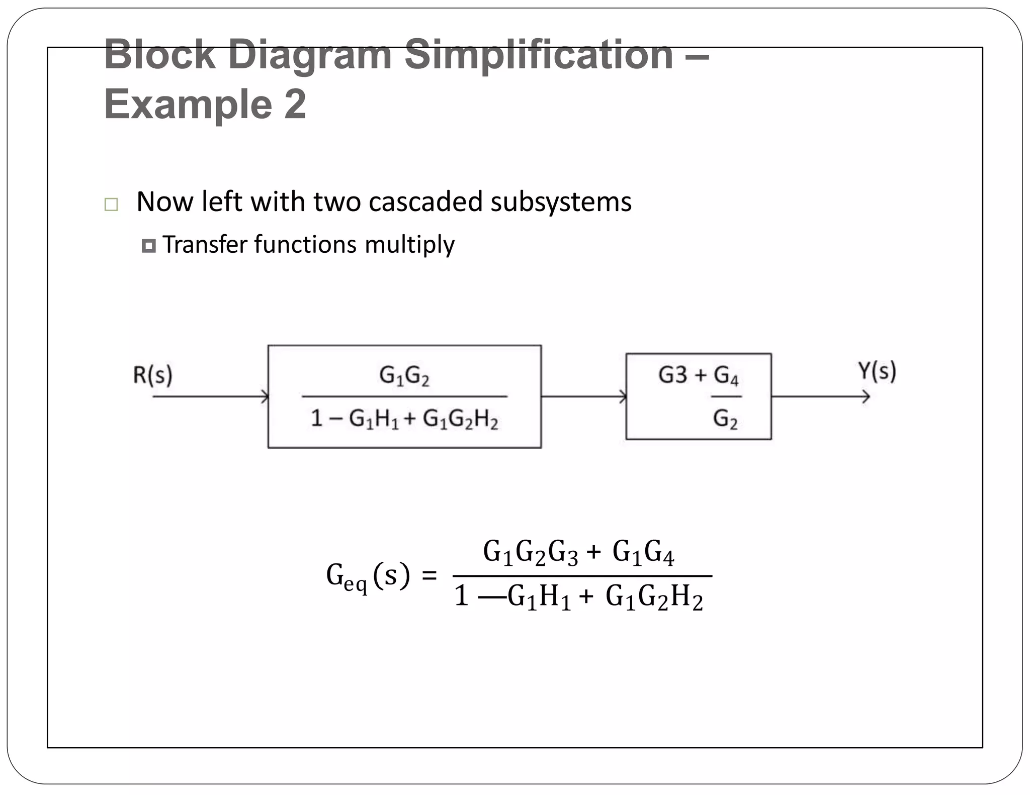
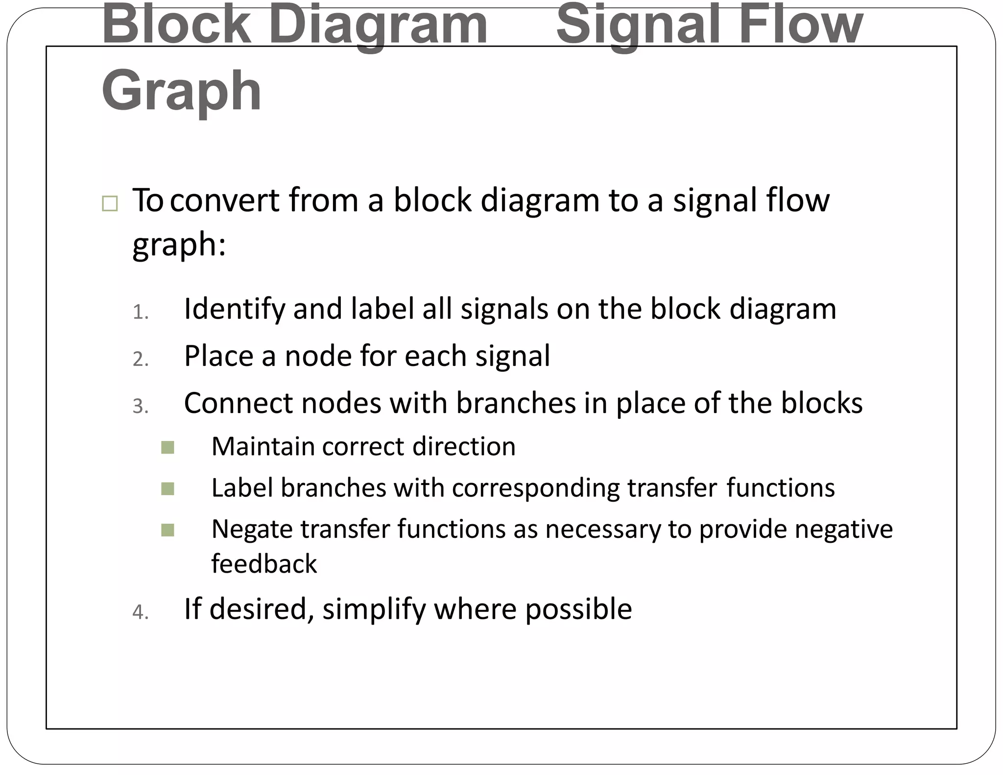
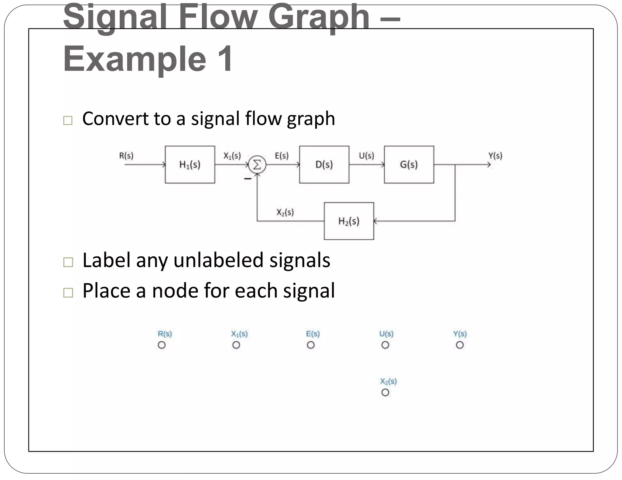
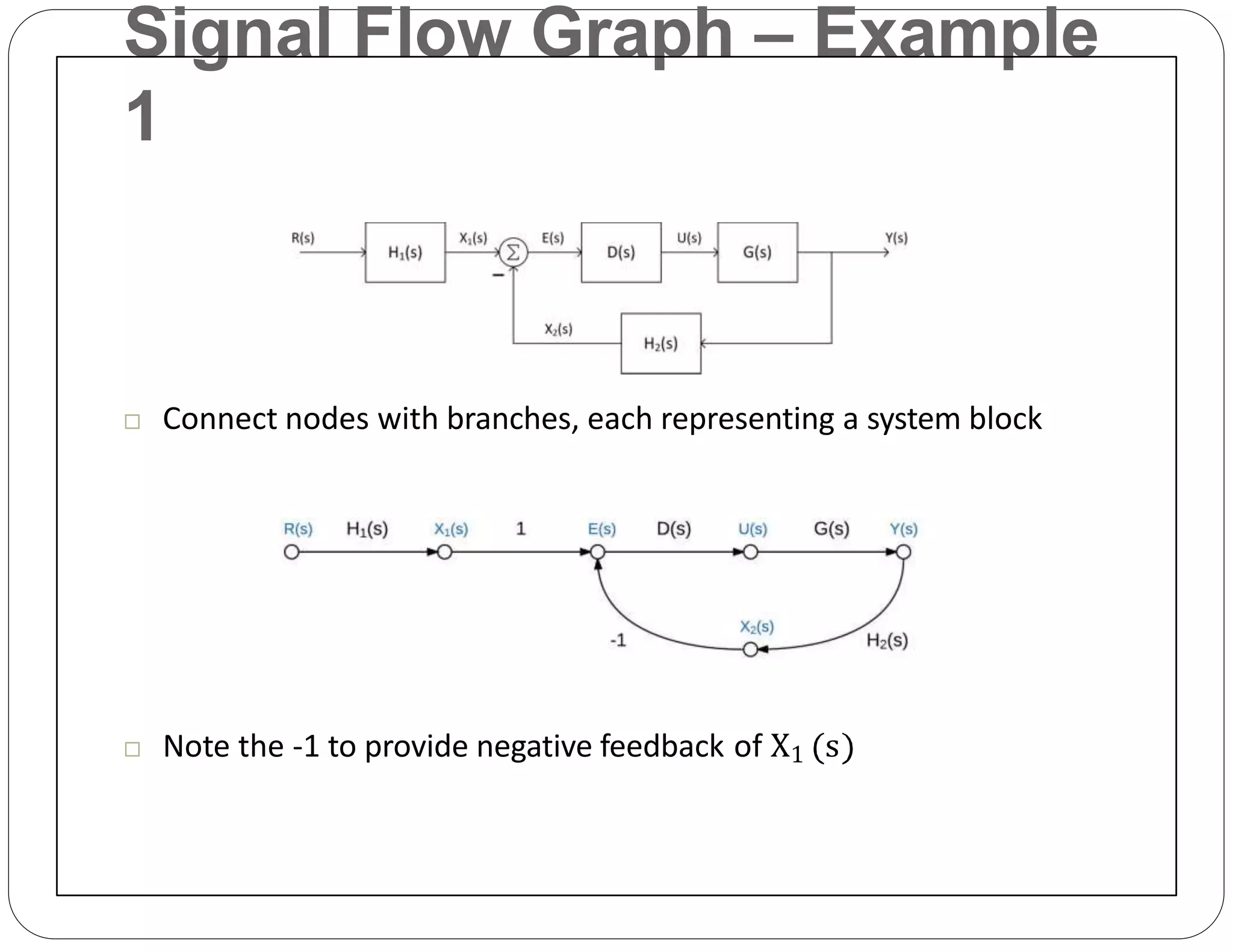
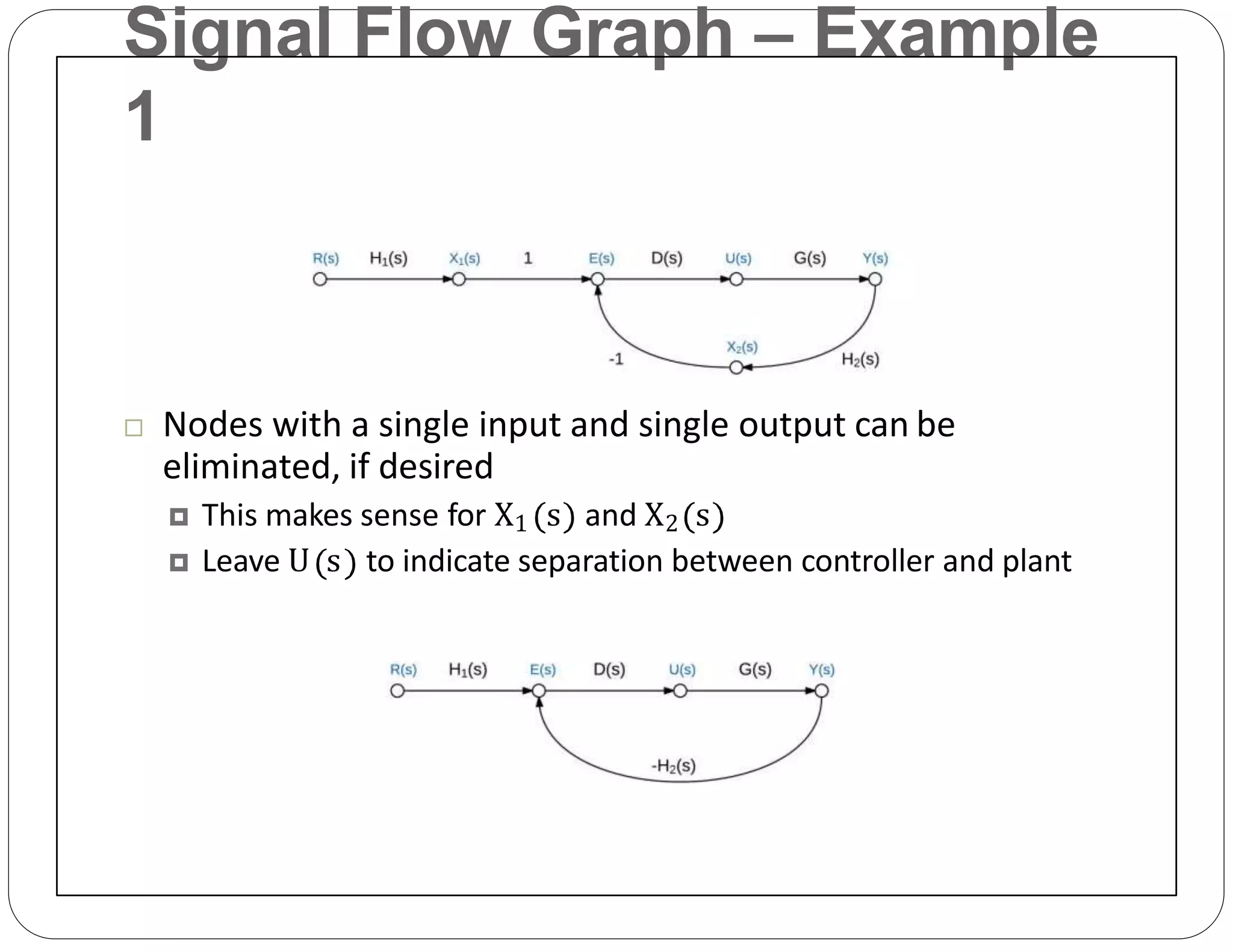
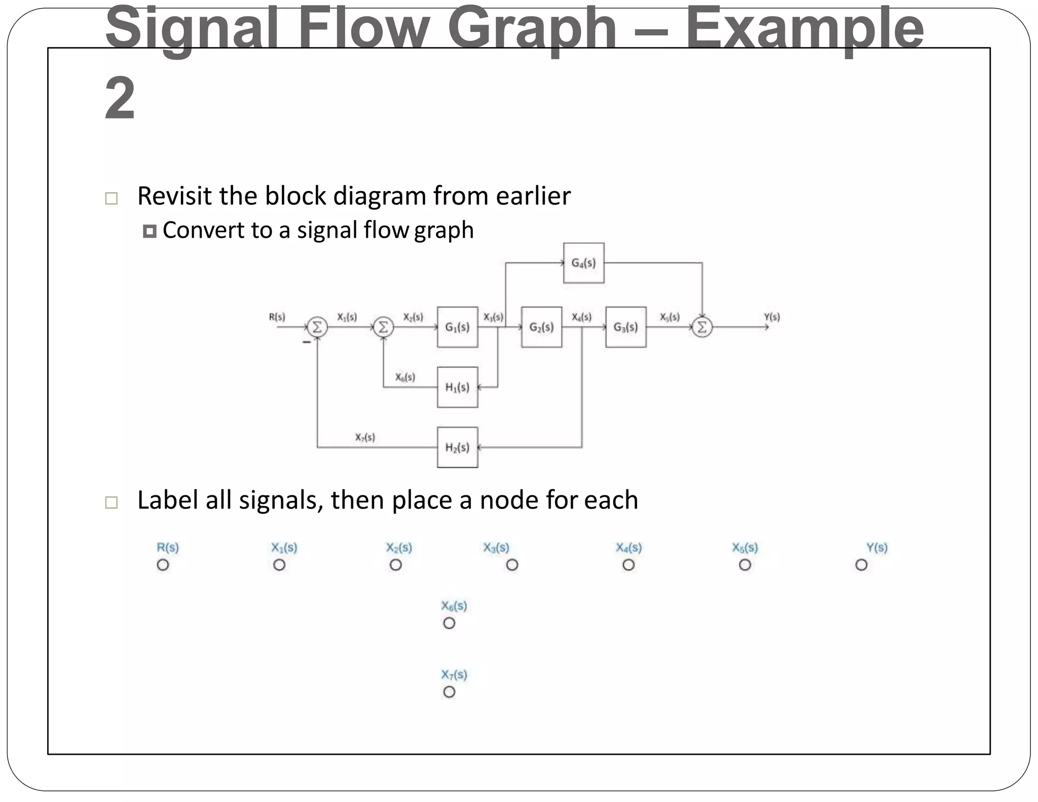
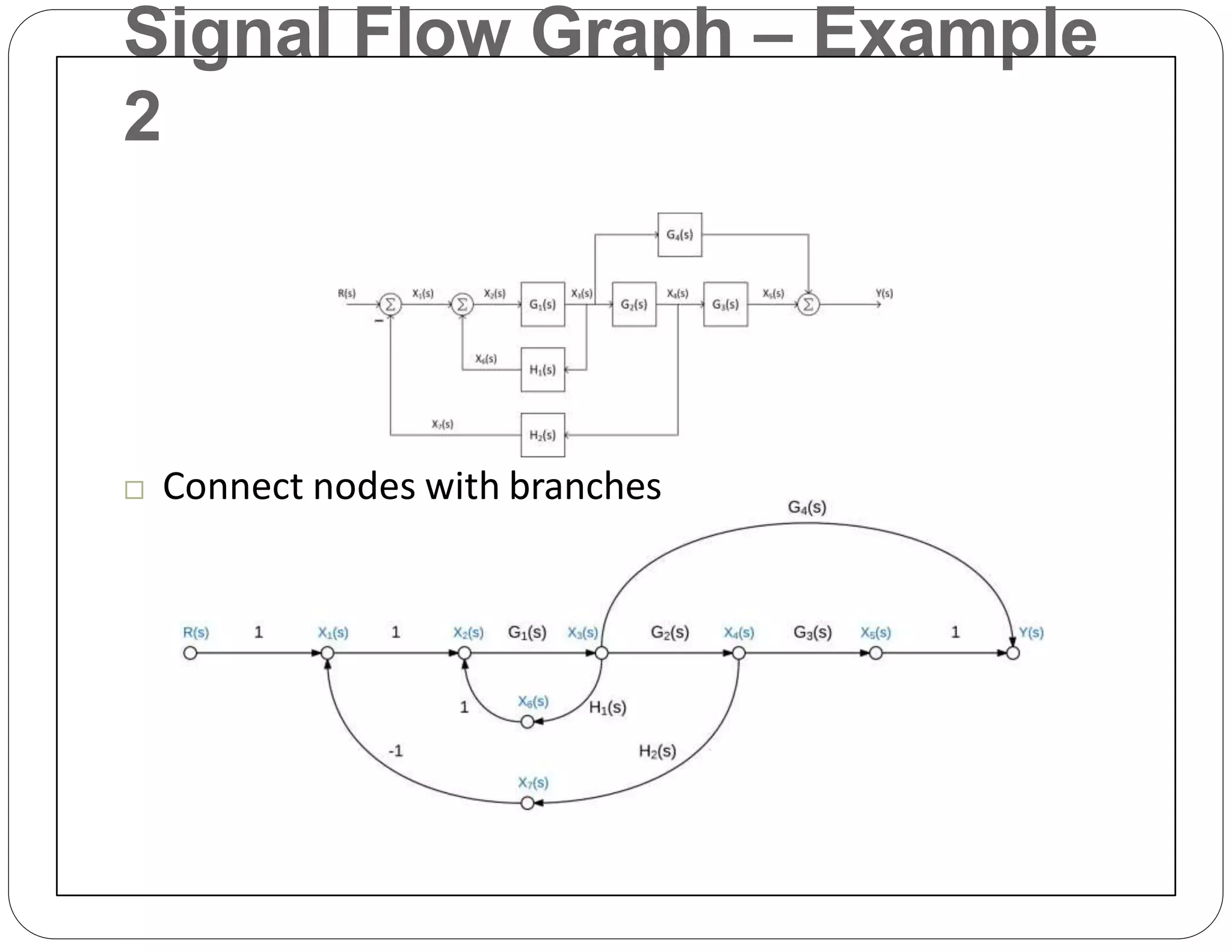
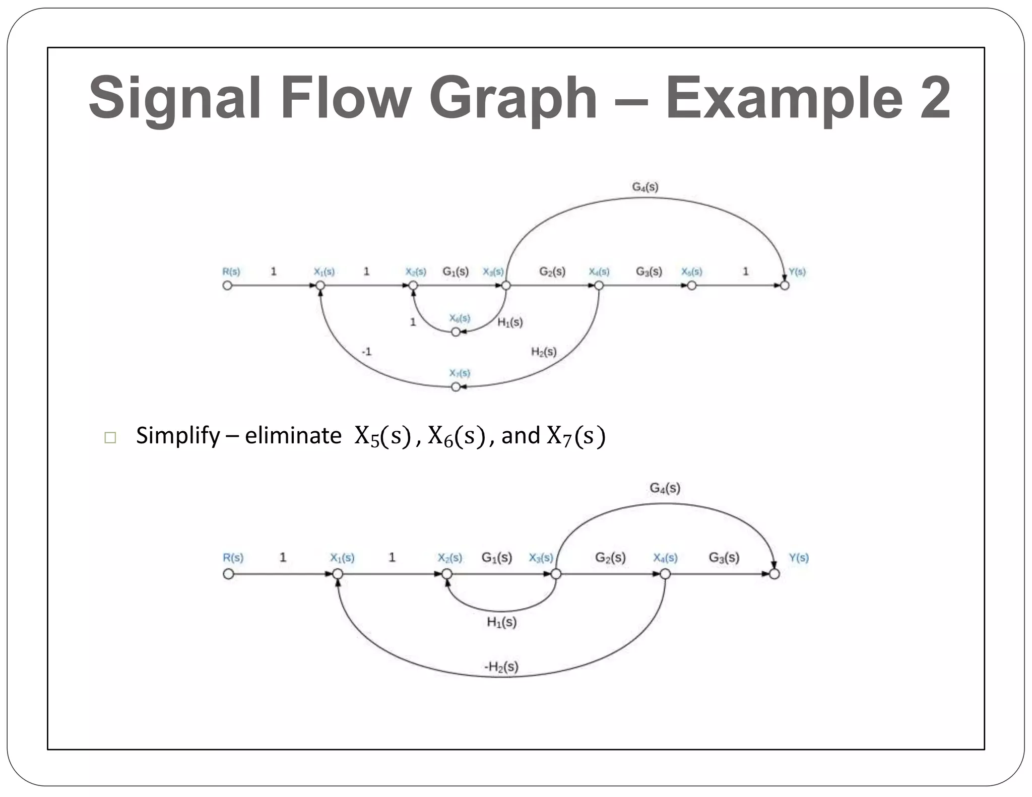
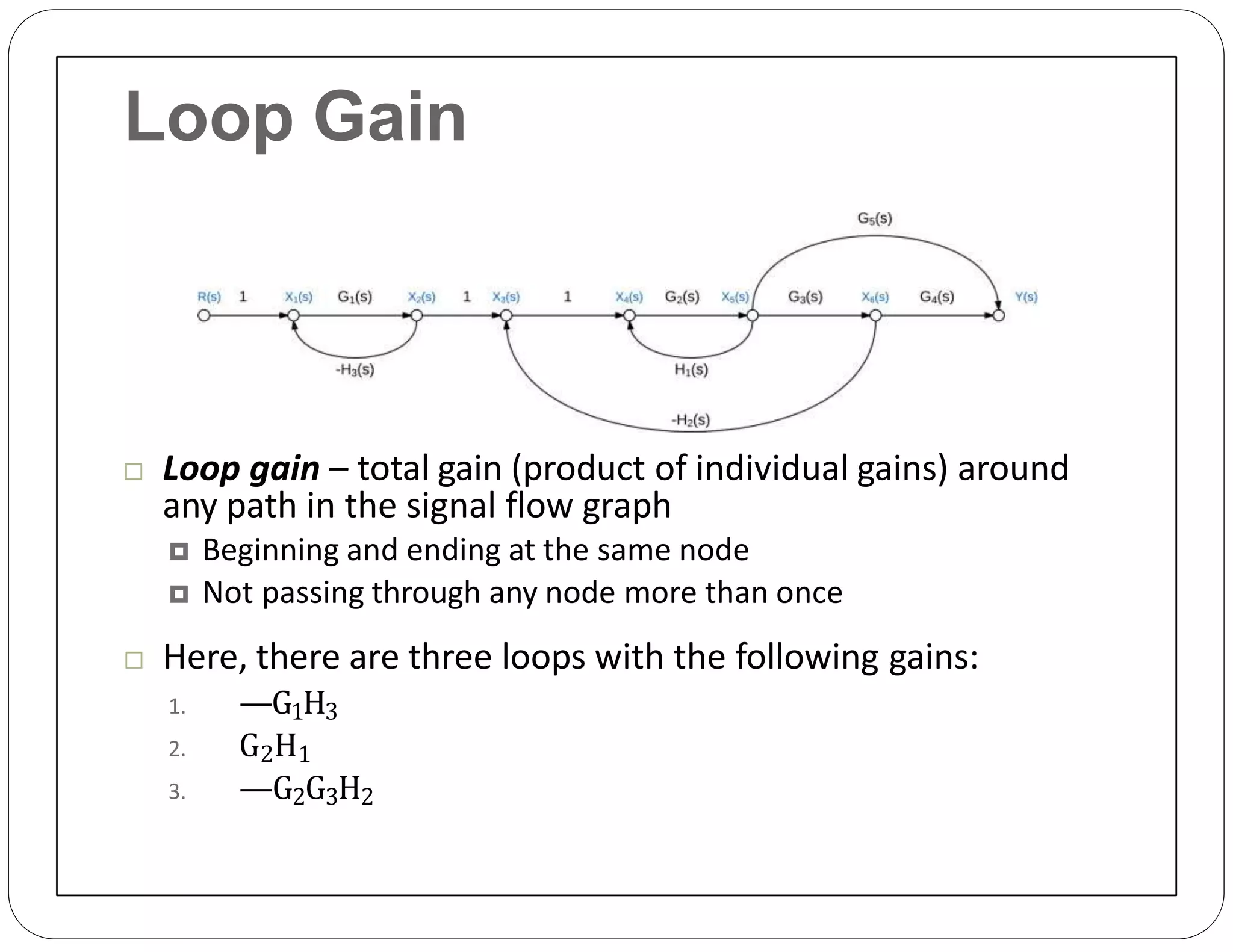
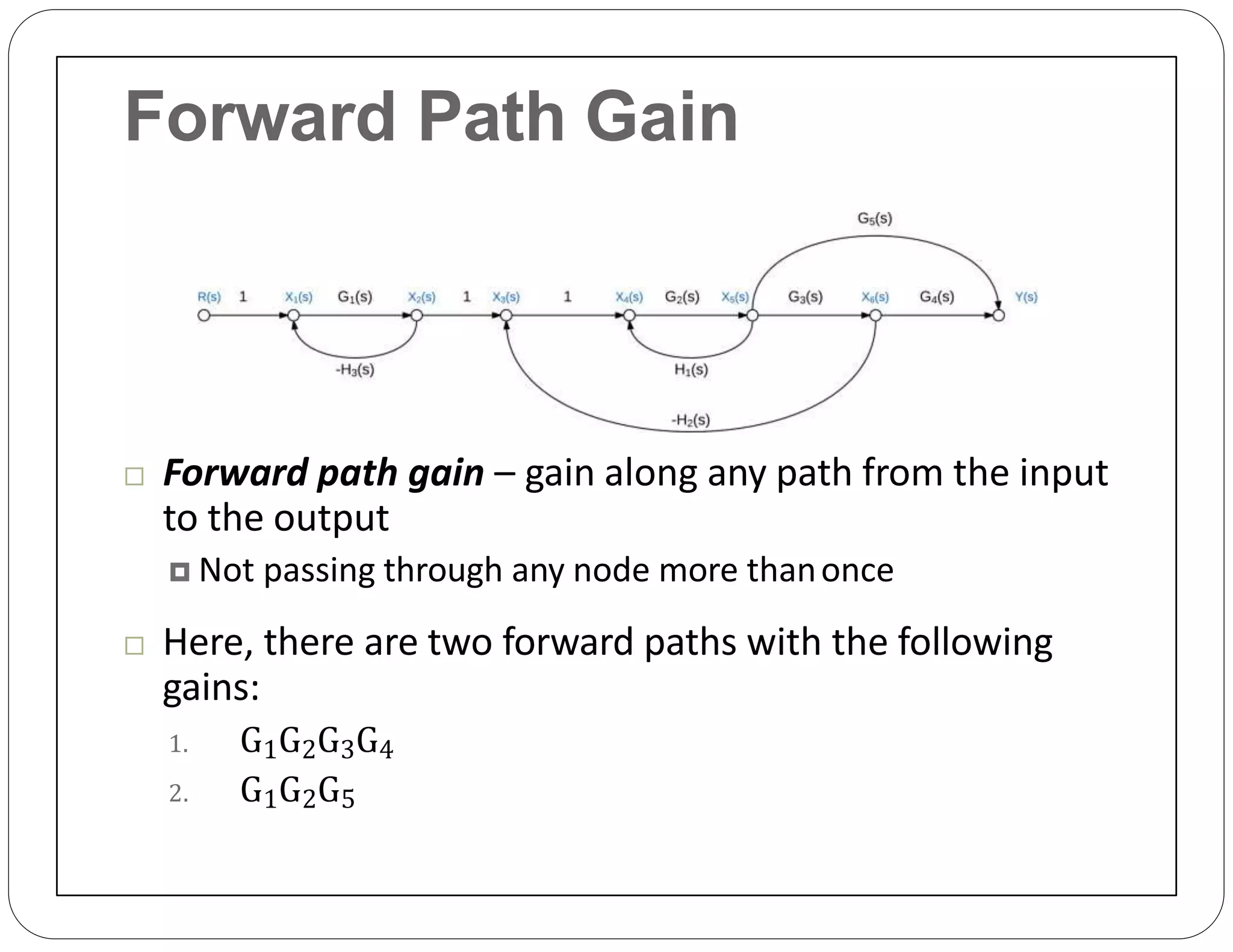
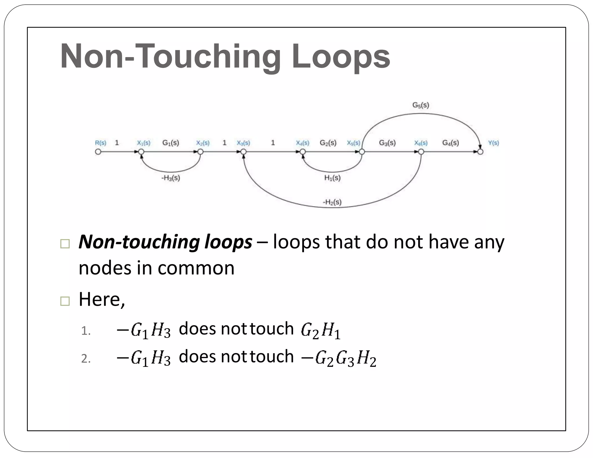
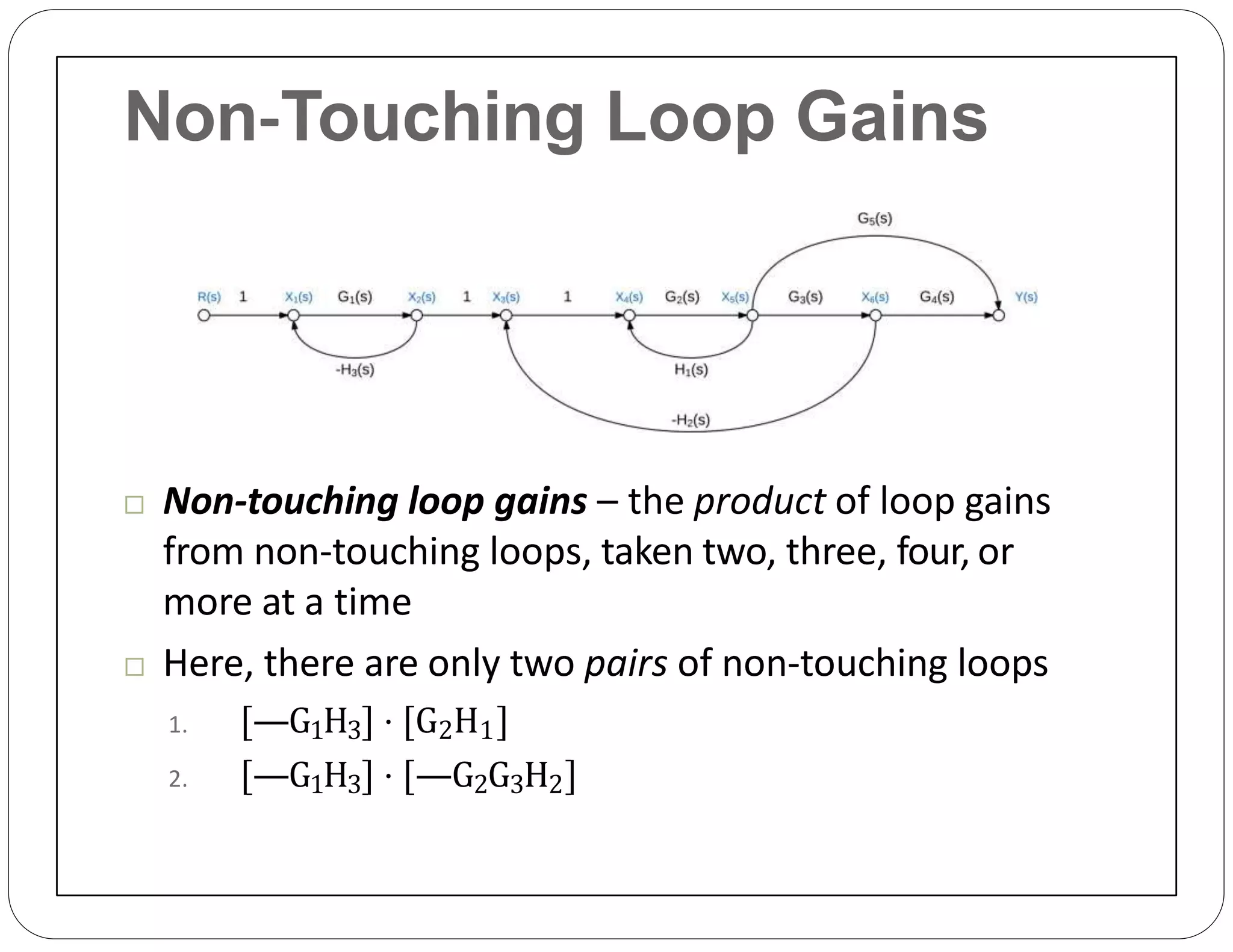
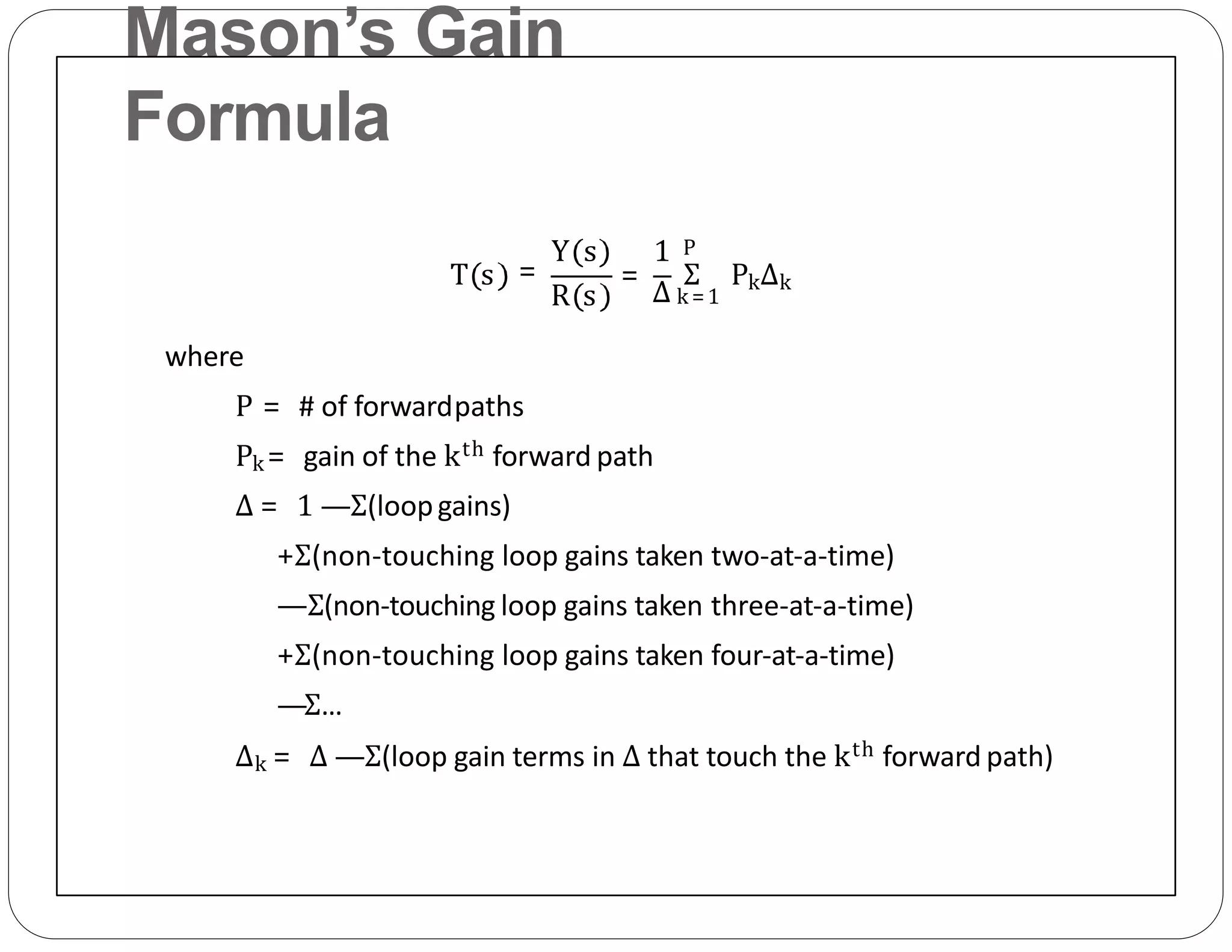
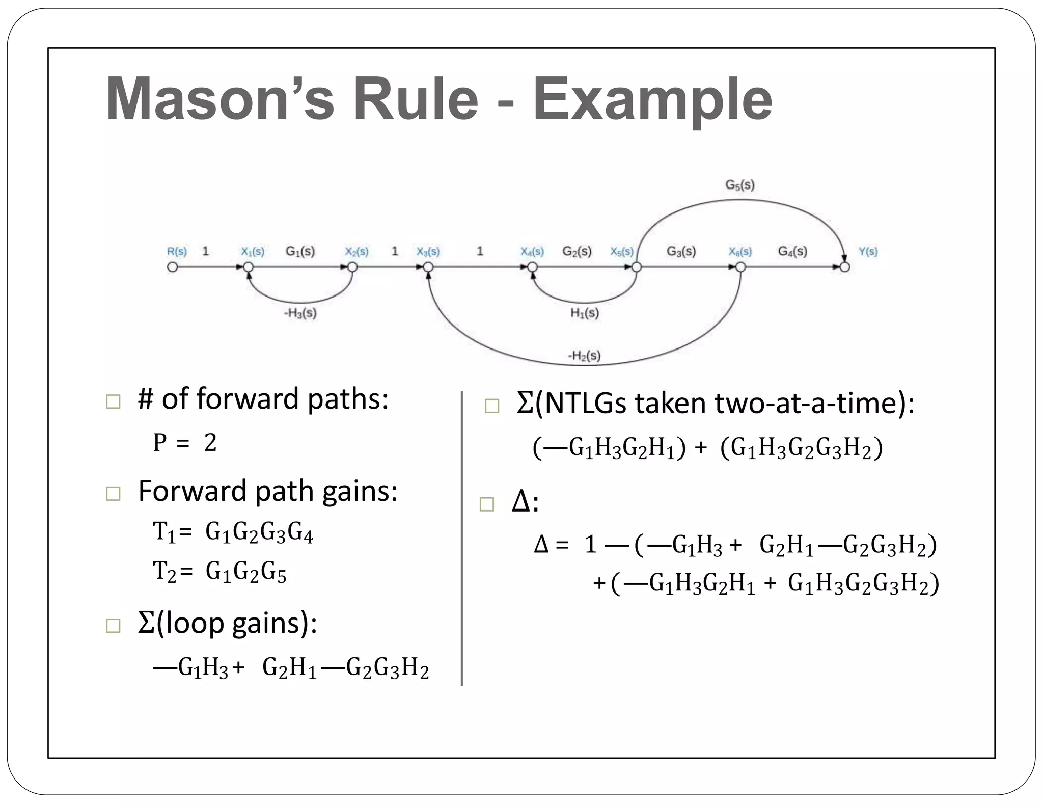
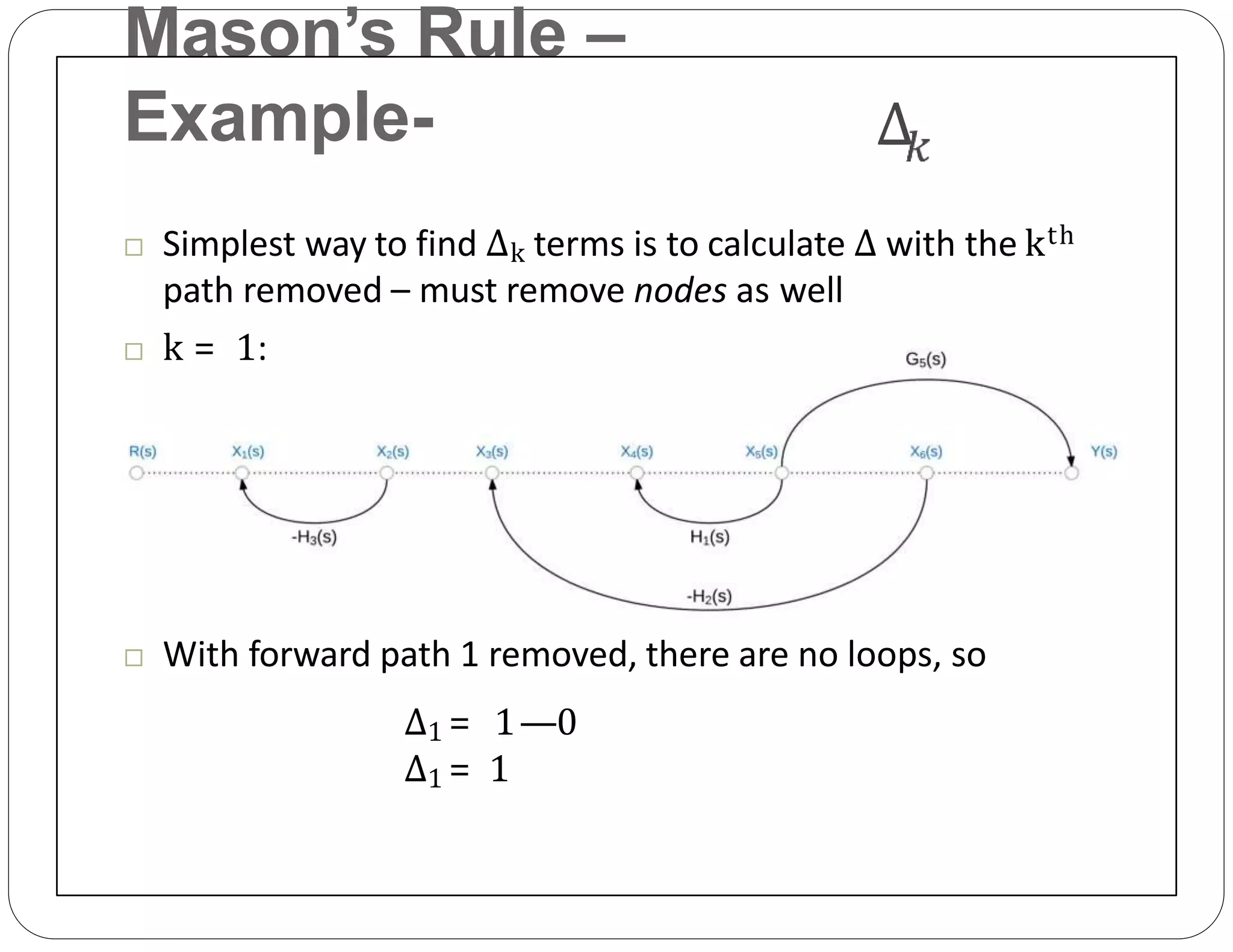
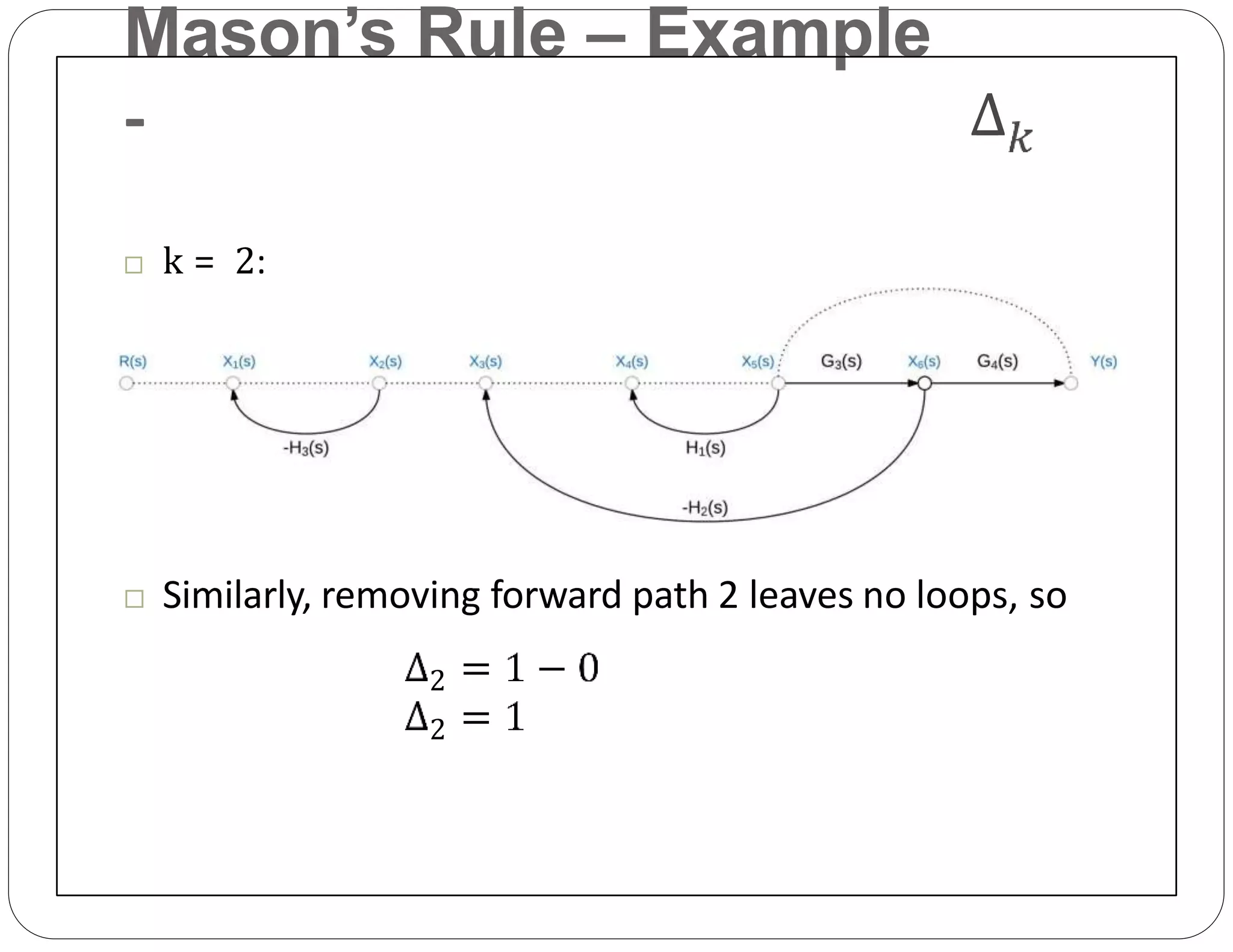
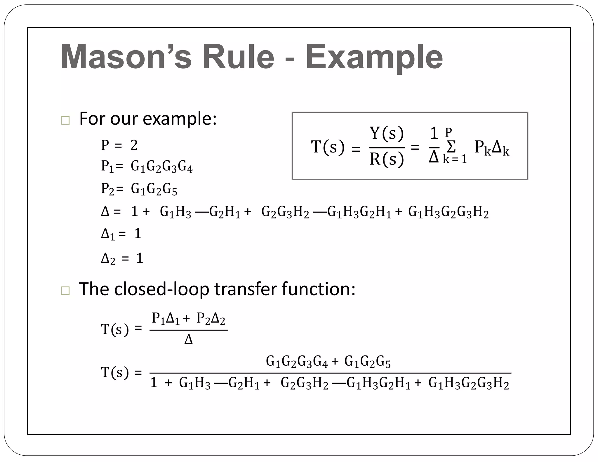
Chapter-2:
BLOCK DIAGRAMS & SIGNAL FLOW GRAPHS
Dr.K.Hussain
Associate Professor & Head
Dept. of EE, SITCOE
Block Diagram Representation
 In the introductory section we saw examples of block diagrams
to represent systems, e.g.:
 Block diagrams consist of
 Blocks – these represent subsystems – typically modeled by, and labeled
with, a transfer function
 Signals – inputs and outputs of blocks – signal direction indicated by
arrows – could be voltage, velocity, force, etc.
 Summing junctions – points were signals are algebraically summed –
subtraction indicated by a negative sign near where the signal joins the
summing junction
Standard Block Diagram
Forms
 The basic input/output relationship for a single block is:
Y s = U s ⋅ G s
 Block diagram blocks can be connected in three basic forms:
 Cascade
 Parallel
 Feedback
 We’ll next look at each of these forms and derive a single‐
block equivalent for each
Cascade Form
 Blocks connected in cascade:
X2 s = X1 s ⋅ G2 sX1 s = U s ⋅ G1 s ,
Y s
Y s
= X2 s ⋅ G3 s = X1 s ⋅ G2 s ⋅ G3 s
= U s ⋅ G1 s ⋅ G2 s ⋅ G3 s = U s ⋅ Geq s
Geq s = G1 s ⋅ G2 s ⋅ G3 s
 The equivalent transfer function of cascaded blocks is the
product of the individual transfer functions
Parallel Form
 Blocks connected in parallel:
X1 s = U s ⋅ G1 s
X2 s = U s ⋅ G2 s
X3 s = U s ⋅ G3 s
Y s = X1 s ± X2 s ± X3 s
Y s = U s ⋅ G1 s ± U s ⋅ G2 s ± U s ⋅ G3 s
Y s = U s G1 s ± G2 s ± G3 s = U s ⋅ Geq s
Geq s = G1 s ± G2 s ± G3 s
 The equivalent transfer function is the sum of the individual
transfer functions:
Feedback Form
 Of obvious interest to us, is the feedback form:
Y s = E s G s
Y s = R s —X s G s
Y s = R s —Y s H s G s
Y s = R s ⋅
Y s 1 + G s H s = R s G s
G s
1 + G s H s
 The closed‐loop transfer function, T s , is
T s ==
Y s G s
R s 1 + G s H s
Feedback Form
 Note that this is negative feedback, for positive feedback:
T s =
G s
1— G s H s
 The G s H s factor in the denominator is the loop gain or open‐loop
transfer function
 The gain from input to output with the feedback path broken is the
forward path gain – here, G s
 In general:
T s =
forward path gain
1 —loop gain
T s =
G s
1 + G s H s
Closed‐Loop Transfer Function ‐ Example
 Calculate the closed‐loop transfer function
 D s and G s are in cascade
 H1 s is in cascade with the feedback system consisting of D s ,
G s , and H2 s
1T s = H s ⋅
D s G s
1 + D s G s H2 s
T s =
H1 s D s G s
1 + D s G s H2 s
Unity‐Feedback
Systems
 We’re often interested in unity‐feedback systems
 Feedback path gain is unity
 Can always reconfigure a system to unity‐feedback form
 Closed‐loop transfer function is:
T s =
D s G s
1 + D s G s
Block Diagram Algebra
 Often want to simplify block diagrams into simpler,
recognizable forms
 Todetermine the equivalent transfer function
 Simplify to instances of the three standard forms,
then simplify those forms
 Move blocks around relative to summing junctions
and pickoff points – simplify to a standard form
 Move blocks forward/backward past summing junctions
 Move blocks forward/backward past pickoff points
Moving Blocks Back Past a Summing
Junction
 The following two block diagrams are equivalent:
Y s = U1 s + U2 s G s = U1 s G s + U2 s G s
Moving Blocks Forward Past a Summing
Junction
 The following two block diagrams are equivalent:
Y s = U1 s G s + U2 s = U1 s + U2 s
1
G s
G s
Moving Blocks Relative to Pickoff
Points
 We can move blocks backward past pickoff points:
 And, we can move them forward past pickoff points:
Block Diagram Simplification –
Example 1
 Rearrange the following into a unity‐feedback system
 Move the feedback block, H s , forward,
past the summing junction
 Add an inverse block on R s to
compensate for the move
 Closed‐loop transfer function:
T s
1 H s G s
1 + G s H s
=
H s
=
G s
1 + G s H s
Block Diagram Simplification –
Example 2
 Find the closed‐loop transfer function of the following
system through block‐diagram simplification
Block Diagram Simplification –
Example 2
 G1 s and H1 s are in feedback form
eqG s =
G1 s
1 —G1 s H1 s
Block Diagram Simplification –
Example 2
 Move G2 s backward past the pickoff point
become a Block from previous step, G2 s , and H2 s
feedback system that can be simplified
Block Diagram Simplification –
Example 2
 Simplify the feedback subsystem
 Note that we’ve dropped the function of s notation, s , forclarity
Geq s =
G1G2
1— G1H1
1 + G1G2H2
1— G1H1
=
G1G2
1— G1H1 + G1G2H2
Block Diagram Simplification –
Example 2
 Simplify the two parallel subsystems
eq 3G s = G +
G4
G2
Block Diagram Simplification –
Example 2
 Now left with two cascaded subsystems
 Transfer functions multiply
eqG s =
G1G2G3 + G1G4
1 —G1H1 + G1G2H2
Block Diagram Simplification –
Example 2
 The equivalent, close‐loop transfer function is
T s =
G1G2G3 + G1G4
1 —G1H1 + G1G2H2
Multiple Input Systems
 Systems often have more than one input
 E.g., reference, R s , and disturbance, W s
 Two transfer functions:
 From reference to output
T s = Y s ⁄ R s
 From disturbance to output
Tw s = Y s /W s
Transfer Function –
Reference
 Find transfer function from to
 A linear system – superposition applies
 Set
Transfer Function –
Reference
to Next, find transfer function from
 Set
 System now becomes:
w
w
Multiple Input Systems
 Two inputs, two transfer functions
T s =
D c G c
and Tw s =
Gw c G c
1+D c G c 1+ D c G c
 is the controller transfer function
 Ultimately, we’ll determine this
w We have control over both and
 What do we want these to be?
 Design
 Design w
for desired performance
for disturbance rejection
Signal Flow Graphs
 An alternative to block diagrams for graphically describing systems
 Signal flow graphs consist of:
 Nodes –represent signals
 Branches –represent system blocks
 Branches labeled with system transfer functions
 Nodes (sometimes) labeled with signal names
 Arrows indicate signal flow direction
 Implicit summation at nodes
 Always a positive sum
 Negative signs associated with branch transfer functions
Block Diagram Signal Flow
Graph
 Toconvert from a block diagram to a signal flow
graph:
1. Identify and label all signals on the block diagram
2. Place a node for each signal
3. Connect nodes with branches in place of the blocks
 Maintain correct direction
 Label branches with corresponding transfer functions
 Negate transfer functions as necessary to provide negative
feedback
4. If desired, simplify where possible
Signal Flow Graph –
Example 1
 Convert to a signal flow graph
 Label any unlabeled signals
 Place a node for each signal
Signal Flow Graph – Example
1
 Connect nodes with branches, each representing a system block
 Note the ‐1 to provide negative feedback of X1 s
Signal Flow Graph – Example
1
 Nodes with a single input and single output can be
eliminated, if desired
 This makes sense for X1 s and X2 s
 Leave U s to indicate separation between controller and plant
Signal Flow Graph – Example
2
 Revisit the block diagram from earlier
 Convert to a signal flow graph
 Label all signals, then place a node for each
Signal Flow Graph – Example
2
 Connect nodes with branches
Signal Flow Graph – Example 2
 Simplify – eliminate X5 s , X6 s , and X7 s
Signal Flow Graphs vs. Block
Diagrams
 Signal flow graphs and block diagrams are
alternative, though equivalent, tools for graphical
representation of interconnected systems
 A generalization (not a rule)
 Signal flow graphs – more often used when dealing
with state‐space system models
 Block diagrams – more often used when dealing with
transfer function system models
Mason’s Rule
 We’ve seen how to reduce a complicated block
diagram to a single input‐to‐output transfer function
 Many successive simplifications
 Mason’s rule provides a formula to calculate the same
overall transfer function
 Single application of the formula
 Can get complicated
 Before presenting the Mason’s rule formula, we need
to define some terminology
Loop Gain
 Loop gain – total gain (product of individual gains) around
any path in the signal flow graph
 Beginning and ending at the same node
 Not passing through any node more than once
 Here, there are three loops with the following gains:
1. —G1H3
2. G2H1
3. —G2G3H2
Forward Path Gain
 Forward path gain – gain along any path from the input
to the output
 Not passing through any node more thanonce
 Here, there are two forward paths with the following
gains:
1. G1G2G3G4
2. G1G2G5
Non‐Touching Loops
 Non‐touching loops – loops that do not have any
nodes in common
 Here,
1.
2.
1
1
3 does nottouch
3 does nottouch
2 1
2 3 2
Non‐Touching Loop Gains
 Non‐touching loop gains – the product of loop gains
from non‐touching loops, taken two, three, four, or
more at a time
 Here, there are only two pairs of non‐touching loops
1. —G1H3 ⋅ G2H1
2. —G1H3 ⋅ —G2G3H2
Mason’s Gain
Formula
T s
R s
=
Y s 1
=
Δ
Σ PkΔk
P
k =1
where
P = # of forwardpaths
Pk = gain of the kth forward path
Δ = 1 —Σ(loopgains)
+Σ(non‐touching loop gains taken two‐at‐a‐time)
—Σ(non‐touching loop gains taken three‐at‐a‐time)
+Σ(non‐touching loop gains taken four‐at‐a‐time)
—Σ…
Δk = Δ —Σ(loop gain terms in Δ that touch the kth forward path)
Mason’s Rule ‐ Example
 # of forward paths:
P = 2
 Forward path gains:
T1= G1G2G3G4
T2= G1G2G5
 Σ(loop gains):
—G1H3+ G2H1—G2G3H2
 Σ(NTLGs taken two‐at‐a‐time):
—G1H3G2H1 + G1H3G2G3H2
 Δ:
Δ = 1 — —G1H3 + G2H1—G2G3H2
+ —G1H3G2H1 + G1H3G2G3H2
Mason’s Rule –
Example-
 Simplest way to find Δk terms is to calculate Δ with the kth
path removed – must remove nodes as well
 k = 1:
 With forward path 1 removed, there are no loops, so
Δ1 = 1—0
Δ1 = 1
Mason’s Rule – Example
‐
 k = 2:
 Similarly, removing forward path 2 leaves no loops, so
2
2
Mason’s Rule ‐ Example
 For our example:
P = 2
P1= G1G2G3G4
P2= G1G2G5
Δ = 1 + G1H3 —G2H1 + G2G3H2 —G1H3G2H1 + G1H3G2G3H2
Δ1 = 1
Δ2 = 1
 The closed‐loop transfer function:
T s =
P1Δ1 + P2Δ2
Δ
T s =
G1G2G3G4 + G1G2G5
1 + G1H3 —G2H1 + G2G3H2 —G1H3G2H1 + G1H3G2G3H2
T s =
R s
Y s 1
=
Δ
Σ PkΔk
P
k =1
Block diagrams and signal flow graphs

Block diagrams and signal flow graphs

  • 1.
    Chapter-2: BLOCK DIAGRAMS &SIGNAL FLOW GRAPHS Dr.K.Hussain Associate Professor & Head Dept. of EE, SITCOE
  • 2.
    Block Diagram Representation In the introductory section we saw examples of block diagrams to represent systems, e.g.:  Block diagrams consist of  Blocks – these represent subsystems – typically modeled by, and labeled with, a transfer function  Signals – inputs and outputs of blocks – signal direction indicated by arrows – could be voltage, velocity, force, etc.  Summing junctions – points were signals are algebraically summed – subtraction indicated by a negative sign near where the signal joins the summing junction
  • 3.
    Standard Block Diagram Forms The basic input/output relationship for a single block is: Y s = U s ⋅ G s  Block diagram blocks can be connected in three basic forms:  Cascade  Parallel  Feedback  We’ll next look at each of these forms and derive a single‐ block equivalent for each
  • 4.
    Cascade Form  Blocksconnected in cascade: X2 s = X1 s ⋅ G2 sX1 s = U s ⋅ G1 s , Y s Y s = X2 s ⋅ G3 s = X1 s ⋅ G2 s ⋅ G3 s = U s ⋅ G1 s ⋅ G2 s ⋅ G3 s = U s ⋅ Geq s Geq s = G1 s ⋅ G2 s ⋅ G3 s  The equivalent transfer function of cascaded blocks is the product of the individual transfer functions
  • 5.
    Parallel Form  Blocksconnected in parallel: X1 s = U s ⋅ G1 s X2 s = U s ⋅ G2 s X3 s = U s ⋅ G3 s Y s = X1 s ± X2 s ± X3 s Y s = U s ⋅ G1 s ± U s ⋅ G2 s ± U s ⋅ G3 s Y s = U s G1 s ± G2 s ± G3 s = U s ⋅ Geq s Geq s = G1 s ± G2 s ± G3 s  The equivalent transfer function is the sum of the individual transfer functions:
  • 6.
    Feedback Form  Ofobvious interest to us, is the feedback form: Y s = E s G s Y s = R s —X s G s Y s = R s —Y s H s G s Y s = R s ⋅ Y s 1 + G s H s = R s G s G s 1 + G s H s  The closed‐loop transfer function, T s , is T s == Y s G s R s 1 + G s H s
  • 7.
    Feedback Form  Notethat this is negative feedback, for positive feedback: T s = G s 1— G s H s  The G s H s factor in the denominator is the loop gain or open‐loop transfer function  The gain from input to output with the feedback path broken is the forward path gain – here, G s  In general: T s = forward path gain 1 —loop gain T s = G s 1 + G s H s
  • 8.
    Closed‐Loop Transfer Function‐ Example  Calculate the closed‐loop transfer function  D s and G s are in cascade  H1 s is in cascade with the feedback system consisting of D s , G s , and H2 s 1T s = H s ⋅ D s G s 1 + D s G s H2 s T s = H1 s D s G s 1 + D s G s H2 s
  • 9.
    Unity‐Feedback Systems  We’re ofteninterested in unity‐feedback systems  Feedback path gain is unity  Can always reconfigure a system to unity‐feedback form  Closed‐loop transfer function is: T s = D s G s 1 + D s G s
  • 10.
    Block Diagram Algebra Often want to simplify block diagrams into simpler, recognizable forms  Todetermine the equivalent transfer function  Simplify to instances of the three standard forms, then simplify those forms  Move blocks around relative to summing junctions and pickoff points – simplify to a standard form  Move blocks forward/backward past summing junctions  Move blocks forward/backward past pickoff points
  • 11.
    Moving Blocks BackPast a Summing Junction  The following two block diagrams are equivalent: Y s = U1 s + U2 s G s = U1 s G s + U2 s G s
  • 12.
    Moving Blocks ForwardPast a Summing Junction  The following two block diagrams are equivalent: Y s = U1 s G s + U2 s = U1 s + U2 s 1 G s G s
  • 13.
    Moving Blocks Relativeto Pickoff Points  We can move blocks backward past pickoff points:  And, we can move them forward past pickoff points:
  • 14.
    Block Diagram Simplification– Example 1  Rearrange the following into a unity‐feedback system  Move the feedback block, H s , forward, past the summing junction  Add an inverse block on R s to compensate for the move  Closed‐loop transfer function: T s 1 H s G s 1 + G s H s = H s = G s 1 + G s H s
  • 15.
    Block Diagram Simplification– Example 2  Find the closed‐loop transfer function of the following system through block‐diagram simplification
  • 16.
    Block Diagram Simplification– Example 2  G1 s and H1 s are in feedback form eqG s = G1 s 1 —G1 s H1 s
  • 17.
    Block Diagram Simplification– Example 2  Move G2 s backward past the pickoff point become a Block from previous step, G2 s , and H2 s feedback system that can be simplified
  • 18.
    Block Diagram Simplification– Example 2  Simplify the feedback subsystem  Note that we’ve dropped the function of s notation, s , forclarity Geq s = G1G2 1— G1H1 1 + G1G2H2 1— G1H1 = G1G2 1— G1H1 + G1G2H2
  • 19.
    Block Diagram Simplification– Example 2  Simplify the two parallel subsystems eq 3G s = G + G4 G2
  • 20.
    Block Diagram Simplification– Example 2  Now left with two cascaded subsystems  Transfer functions multiply eqG s = G1G2G3 + G1G4 1 —G1H1 + G1G2H2
  • 21.
    Block Diagram Simplification– Example 2  The equivalent, close‐loop transfer function is T s = G1G2G3 + G1G4 1 —G1H1 + G1G2H2
  • 22.
    Multiple Input Systems Systems often have more than one input  E.g., reference, R s , and disturbance, W s  Two transfer functions:  From reference to output T s = Y s ⁄ R s  From disturbance to output Tw s = Y s /W s
  • 23.
    Transfer Function – Reference Find transfer function from to  A linear system – superposition applies  Set
  • 24.
    Transfer Function – Reference toNext, find transfer function from  Set  System now becomes: w w
  • 25.
    Multiple Input Systems Two inputs, two transfer functions T s = D c G c and Tw s = Gw c G c 1+D c G c 1+ D c G c  is the controller transfer function  Ultimately, we’ll determine this w We have control over both and  What do we want these to be?  Design  Design w for desired performance for disturbance rejection
  • 26.
    Signal Flow Graphs An alternative to block diagrams for graphically describing systems  Signal flow graphs consist of:  Nodes –represent signals  Branches –represent system blocks  Branches labeled with system transfer functions  Nodes (sometimes) labeled with signal names  Arrows indicate signal flow direction  Implicit summation at nodes  Always a positive sum  Negative signs associated with branch transfer functions
  • 27.
    Block Diagram SignalFlow Graph  Toconvert from a block diagram to a signal flow graph: 1. Identify and label all signals on the block diagram 2. Place a node for each signal 3. Connect nodes with branches in place of the blocks  Maintain correct direction  Label branches with corresponding transfer functions  Negate transfer functions as necessary to provide negative feedback 4. If desired, simplify where possible
  • 28.
    Signal Flow Graph– Example 1  Convert to a signal flow graph  Label any unlabeled signals  Place a node for each signal
  • 29.
    Signal Flow Graph– Example 1  Connect nodes with branches, each representing a system block  Note the ‐1 to provide negative feedback of X1 s
  • 30.
    Signal Flow Graph– Example 1  Nodes with a single input and single output can be eliminated, if desired  This makes sense for X1 s and X2 s  Leave U s to indicate separation between controller and plant
  • 31.
    Signal Flow Graph– Example 2  Revisit the block diagram from earlier  Convert to a signal flow graph  Label all signals, then place a node for each
  • 32.
    Signal Flow Graph– Example 2  Connect nodes with branches
  • 33.
    Signal Flow Graph– Example 2  Simplify – eliminate X5 s , X6 s , and X7 s
  • 34.
    Signal Flow Graphsvs. Block Diagrams  Signal flow graphs and block diagrams are alternative, though equivalent, tools for graphical representation of interconnected systems  A generalization (not a rule)  Signal flow graphs – more often used when dealing with state‐space system models  Block diagrams – more often used when dealing with transfer function system models
  • 35.
    Mason’s Rule  We’veseen how to reduce a complicated block diagram to a single input‐to‐output transfer function  Many successive simplifications  Mason’s rule provides a formula to calculate the same overall transfer function  Single application of the formula  Can get complicated  Before presenting the Mason’s rule formula, we need to define some terminology
  • 36.
    Loop Gain  Loopgain – total gain (product of individual gains) around any path in the signal flow graph  Beginning and ending at the same node  Not passing through any node more than once  Here, there are three loops with the following gains: 1. —G1H3 2. G2H1 3. —G2G3H2
  • 37.
    Forward Path Gain Forward path gain – gain along any path from the input to the output  Not passing through any node more thanonce  Here, there are two forward paths with the following gains: 1. G1G2G3G4 2. G1G2G5
  • 38.
    Non‐Touching Loops  Non‐touchingloops – loops that do not have any nodes in common  Here, 1. 2. 1 1 3 does nottouch 3 does nottouch 2 1 2 3 2
  • 39.
    Non‐Touching Loop Gains Non‐touching loop gains – the product of loop gains from non‐touching loops, taken two, three, four, or more at a time  Here, there are only two pairs of non‐touching loops 1. —G1H3 ⋅ G2H1 2. —G1H3 ⋅ —G2G3H2
  • 40.
    Mason’s Gain Formula T s Rs = Y s 1 = Δ Σ PkΔk P k =1 where P = # of forwardpaths Pk = gain of the kth forward path Δ = 1 —Σ(loopgains) +Σ(non‐touching loop gains taken two‐at‐a‐time) —Σ(non‐touching loop gains taken three‐at‐a‐time) +Σ(non‐touching loop gains taken four‐at‐a‐time) —Σ… Δk = Δ —Σ(loop gain terms in Δ that touch the kth forward path)
  • 41.
    Mason’s Rule ‐Example  # of forward paths: P = 2  Forward path gains: T1= G1G2G3G4 T2= G1G2G5  Σ(loop gains): —G1H3+ G2H1—G2G3H2  Σ(NTLGs taken two‐at‐a‐time): —G1H3G2H1 + G1H3G2G3H2  Δ: Δ = 1 — —G1H3 + G2H1—G2G3H2 + —G1H3G2H1 + G1H3G2G3H2
  • 42.
    Mason’s Rule – Example- Simplest way to find Δk terms is to calculate Δ with the kth path removed – must remove nodes as well  k = 1:  With forward path 1 removed, there are no loops, so Δ1 = 1—0 Δ1 = 1
  • 43.
    Mason’s Rule –Example ‐  k = 2:  Similarly, removing forward path 2 leaves no loops, so 2 2
  • 44.
    Mason’s Rule ‐Example  For our example: P = 2 P1= G1G2G3G4 P2= G1G2G5 Δ = 1 + G1H3 —G2H1 + G2G3H2 —G1H3G2H1 + G1H3G2G3H2 Δ1 = 1 Δ2 = 1  The closed‐loop transfer function: T s = P1Δ1 + P2Δ2 Δ T s = G1G2G3G4 + G1G2G5 1 + G1H3 —G2H1 + G2G3H2 —G1H3G2H1 + G1H3G2G3H2 T s = R s Y s 1 = Δ Σ PkΔk P k =1