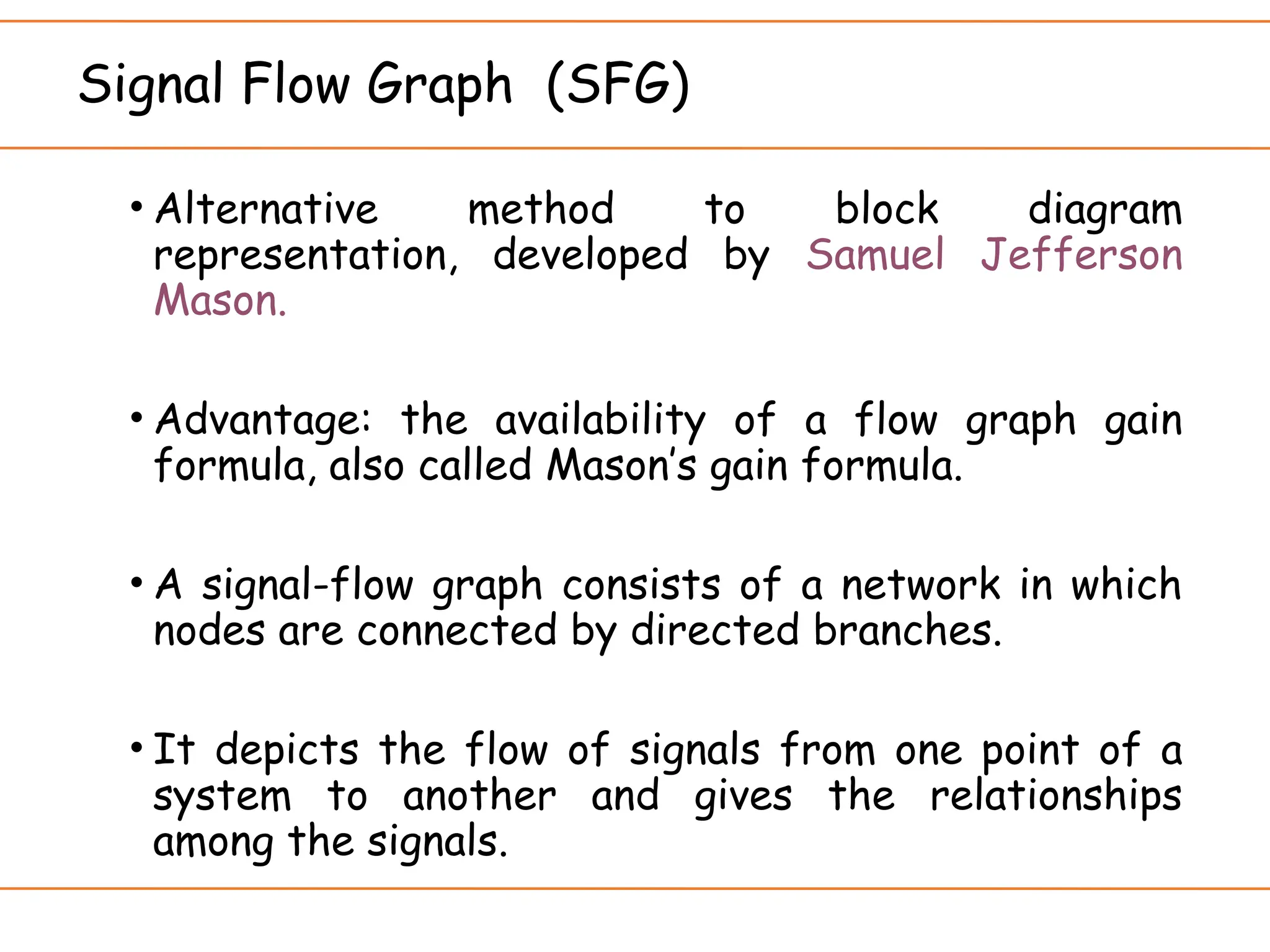
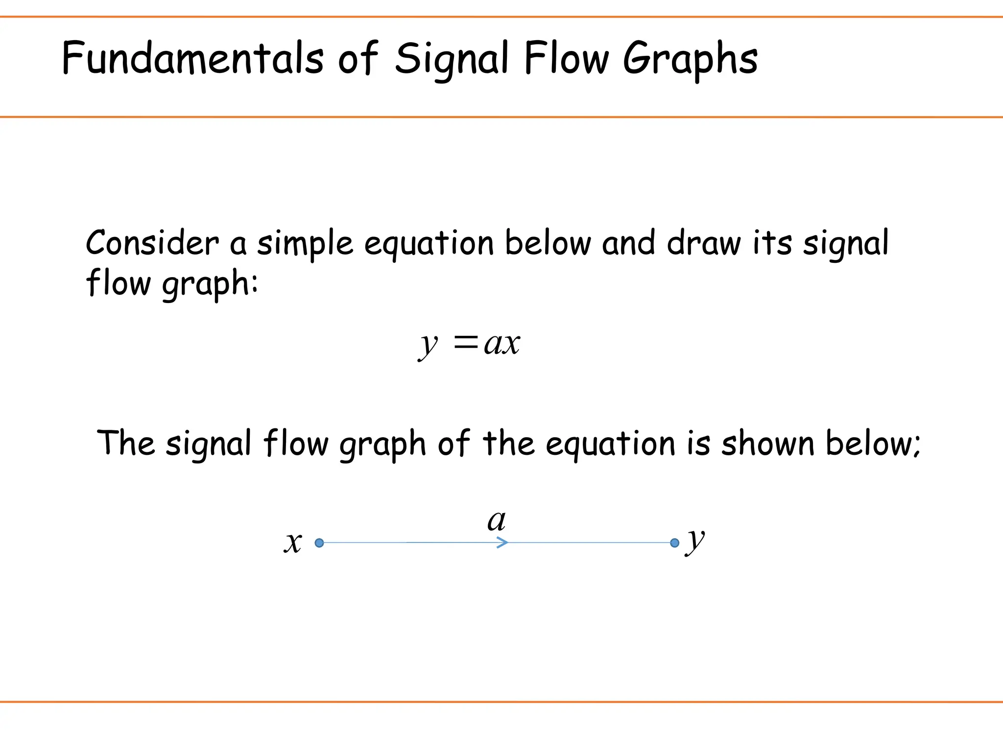
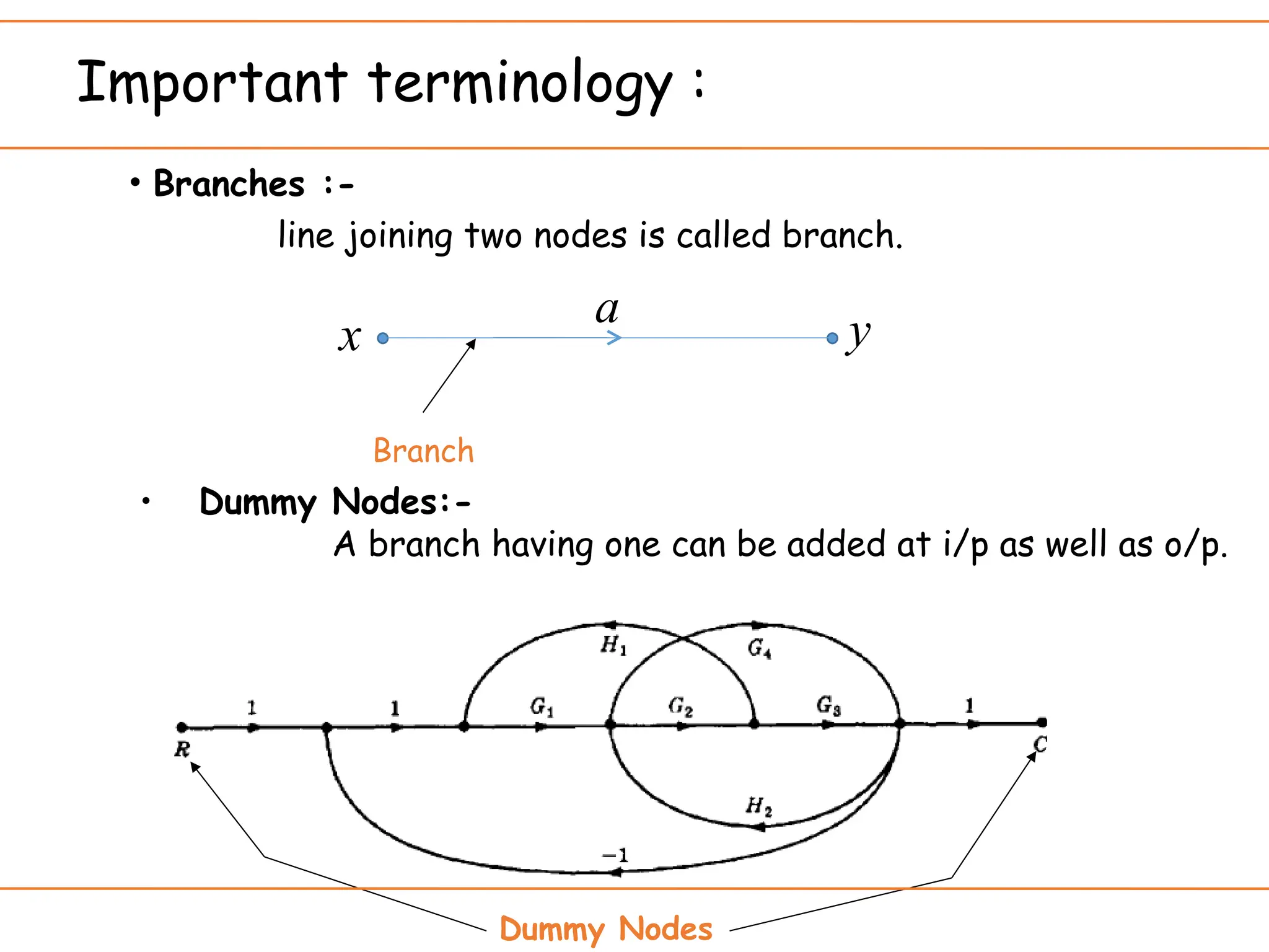
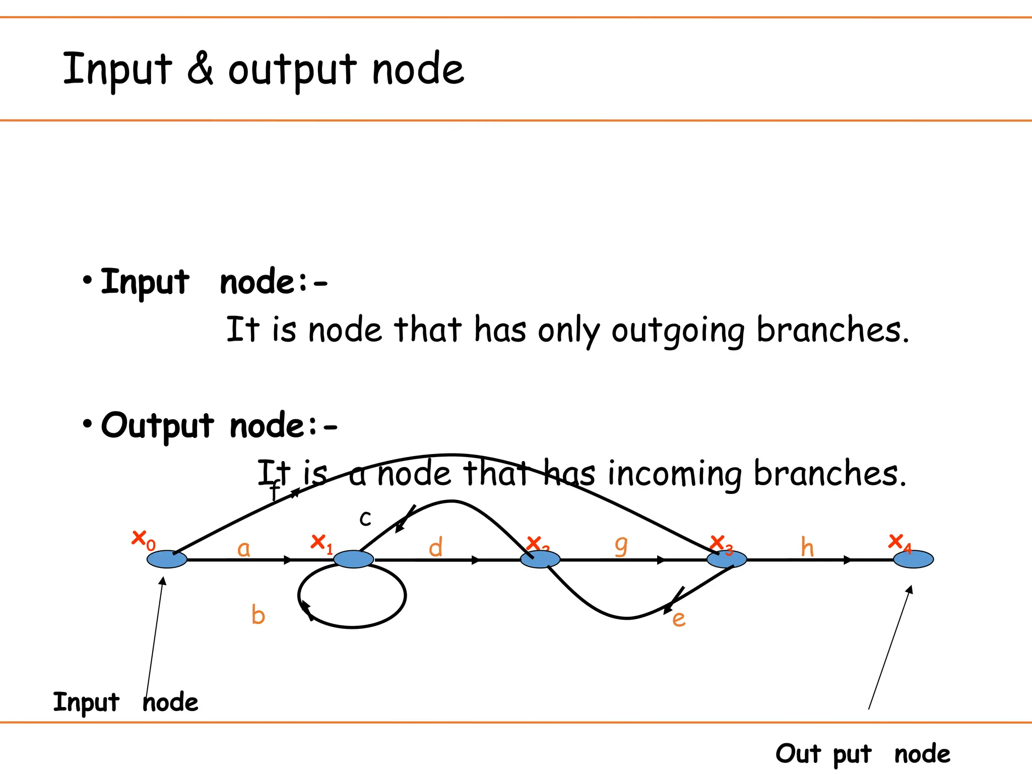
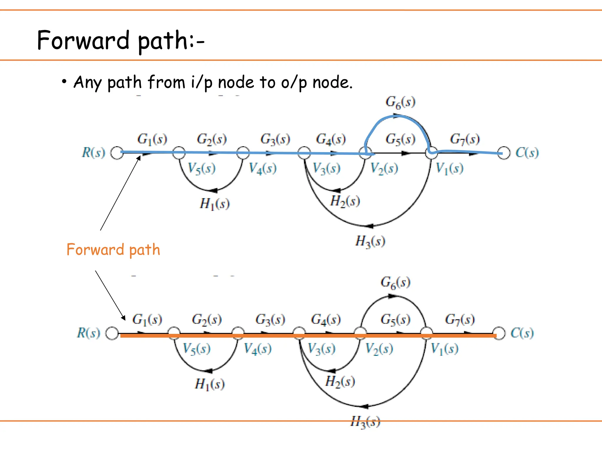
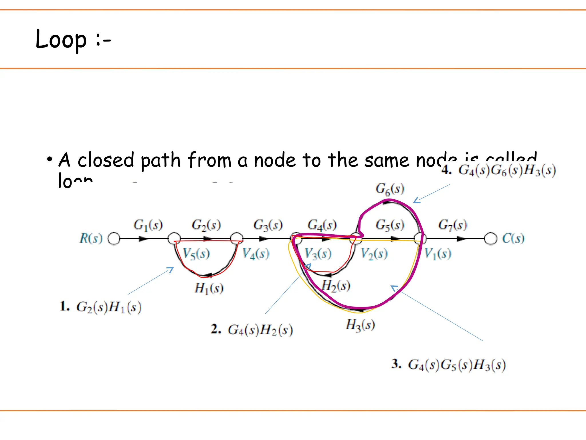
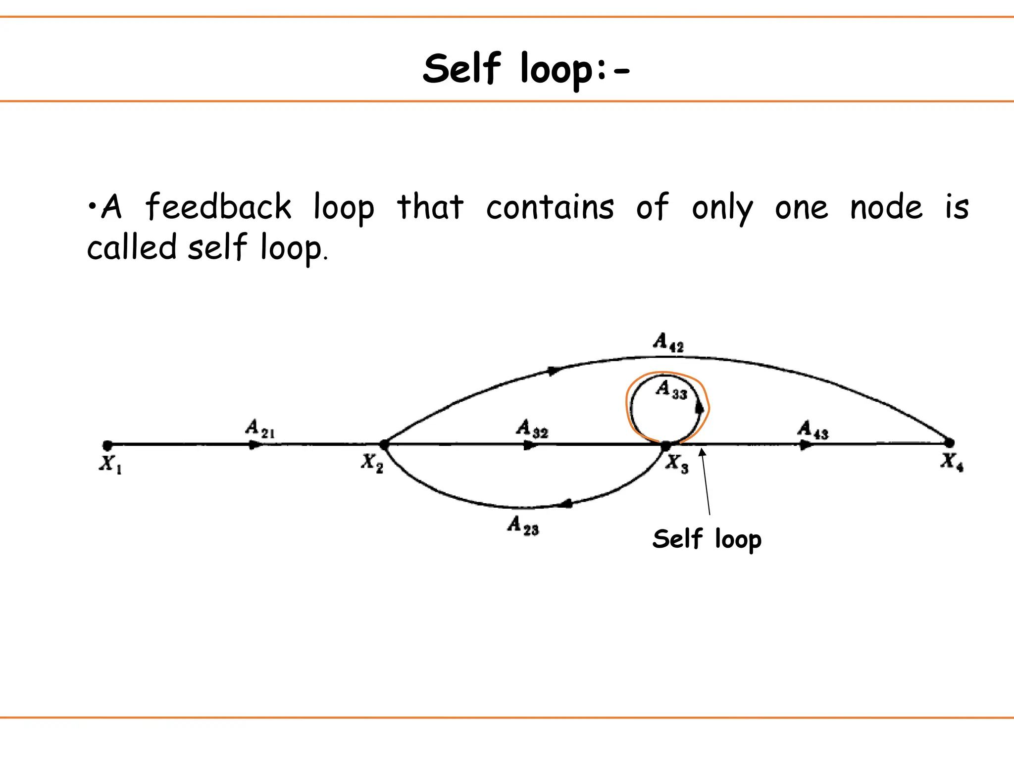
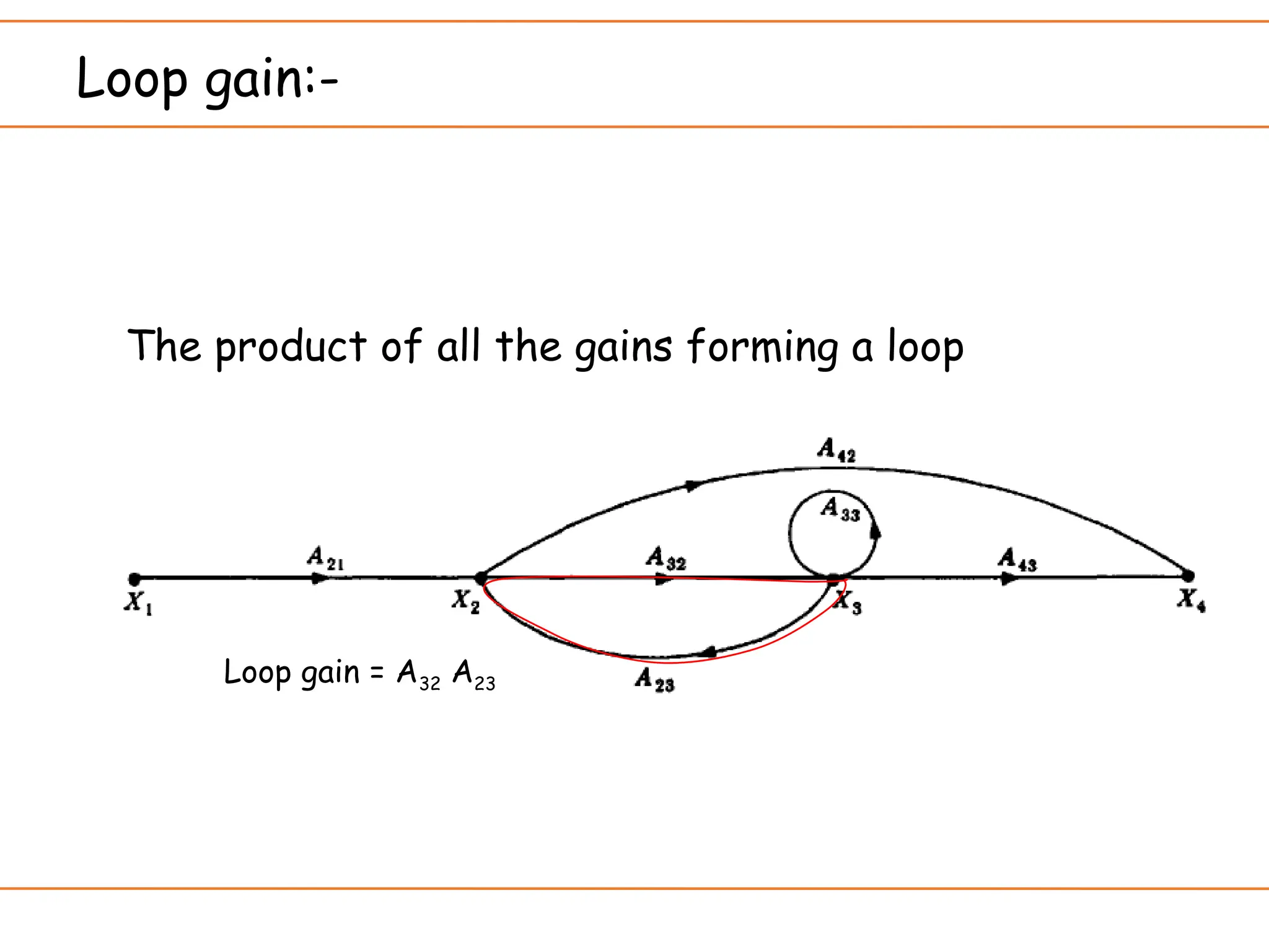
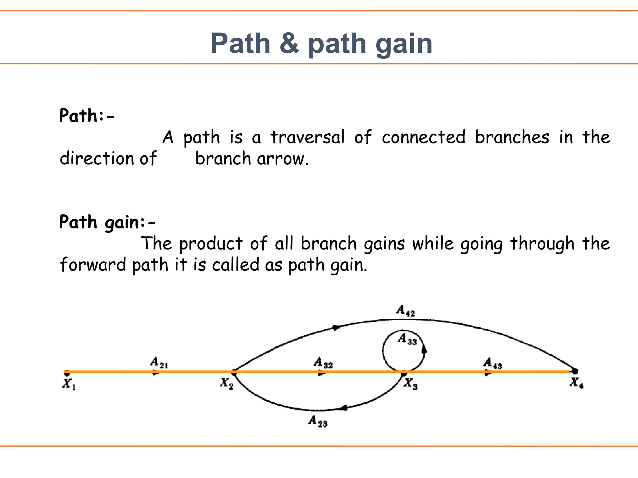
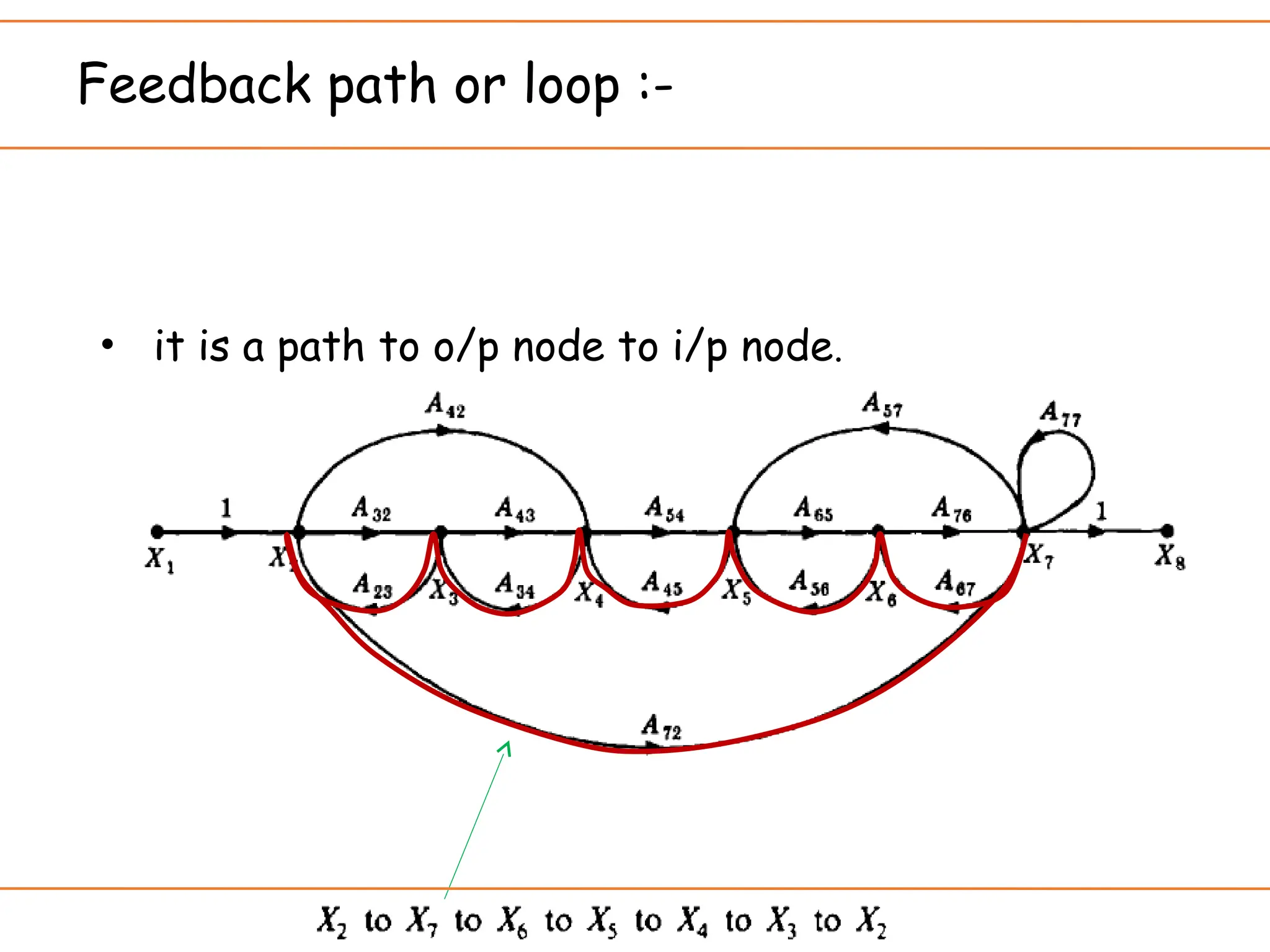
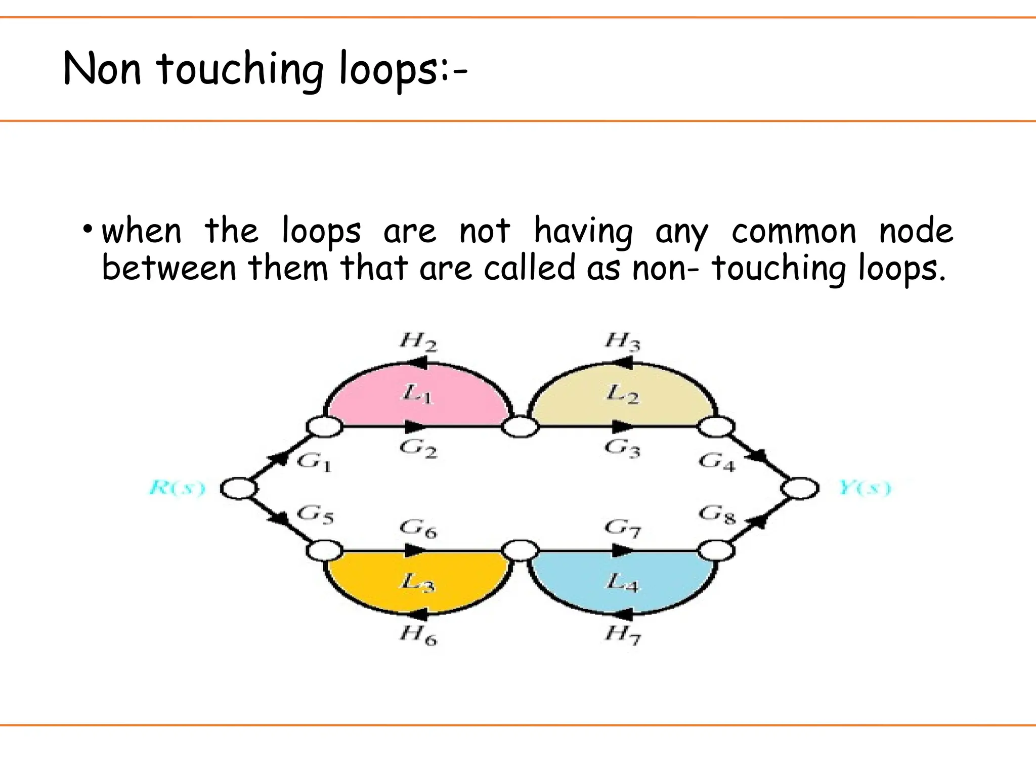
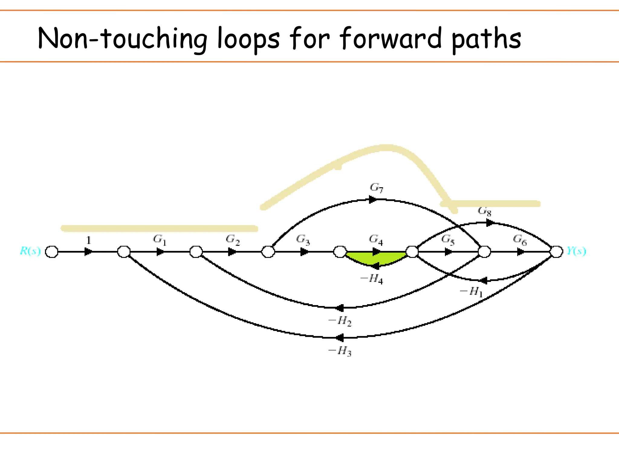
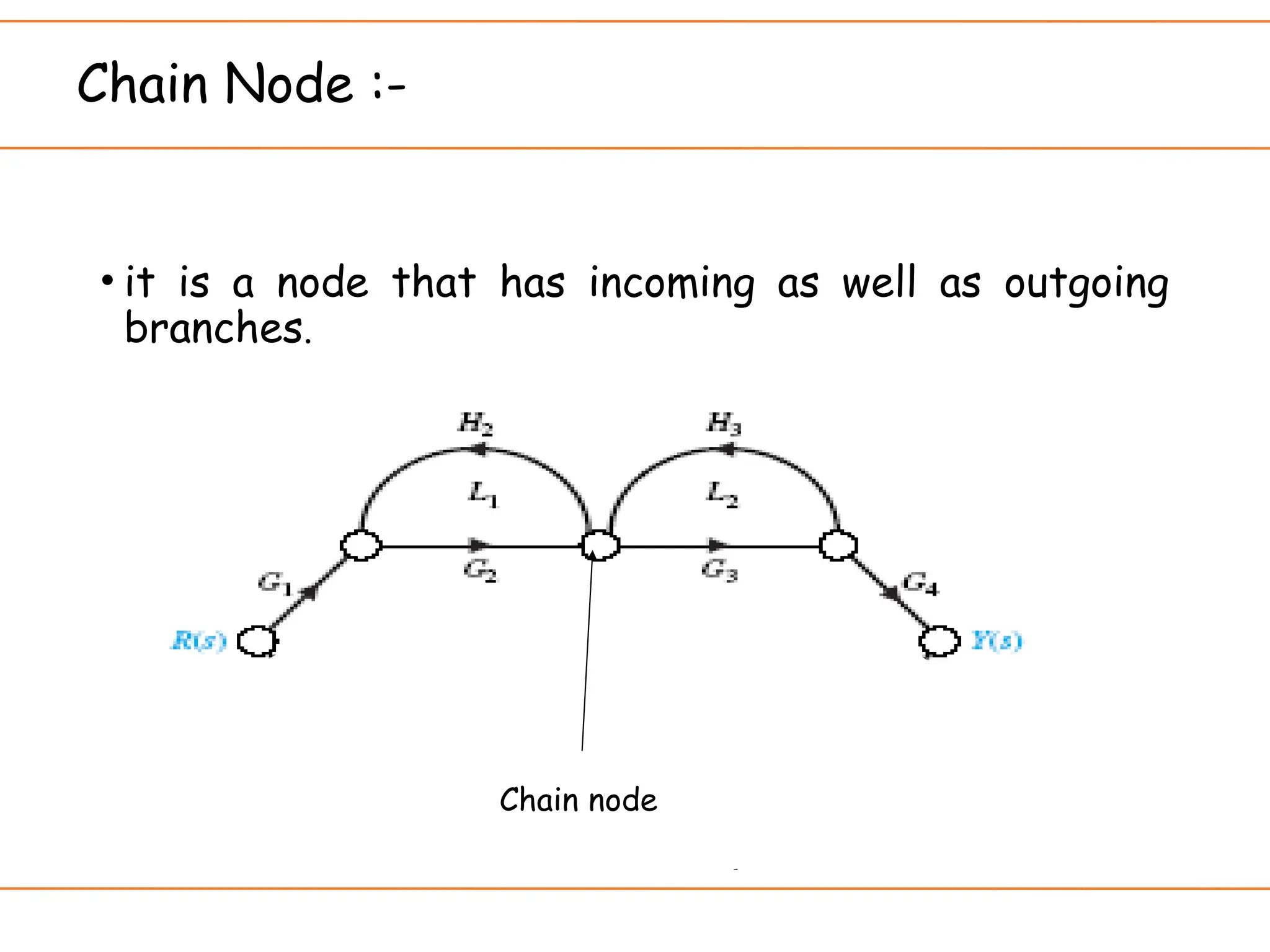
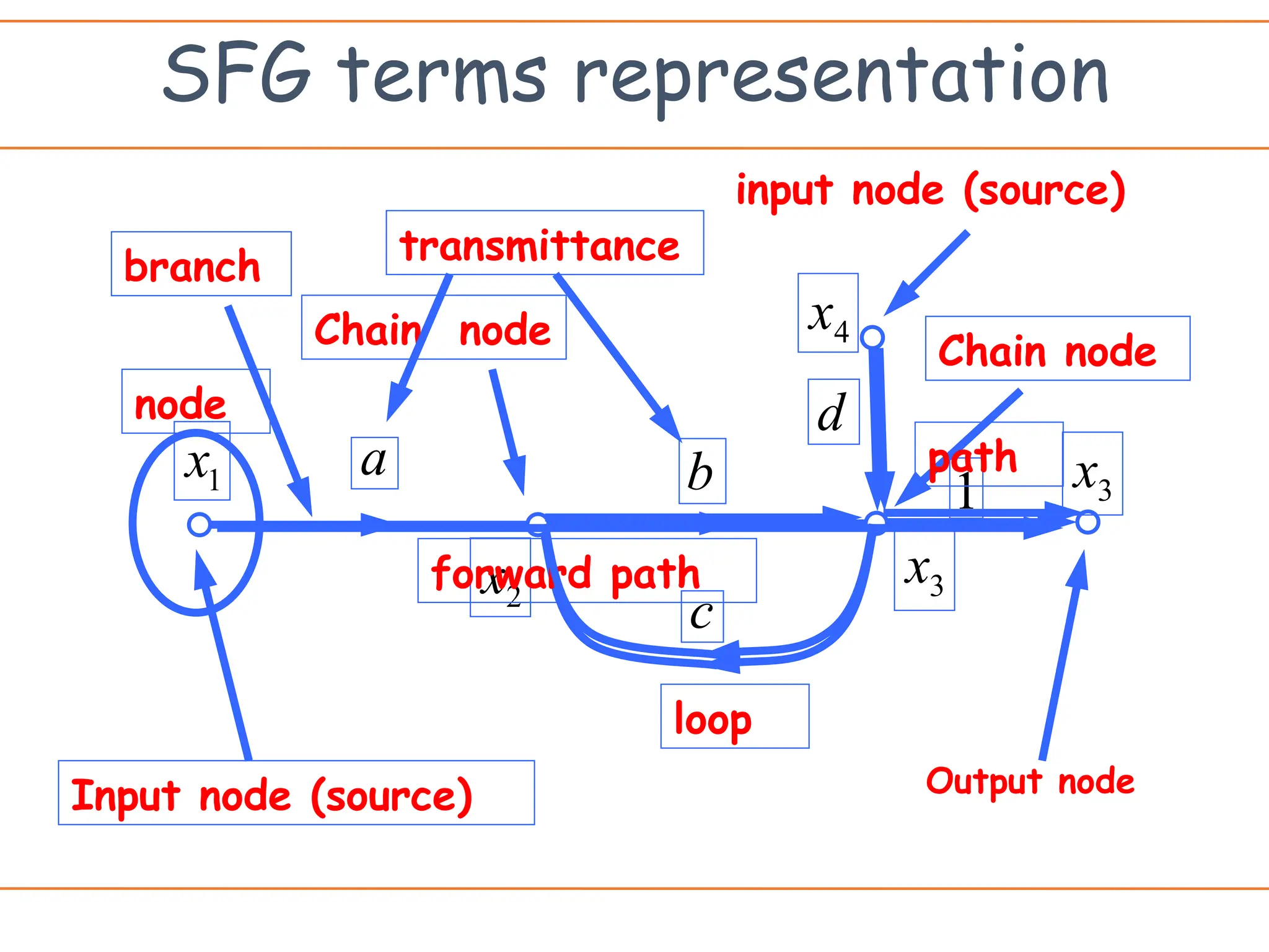
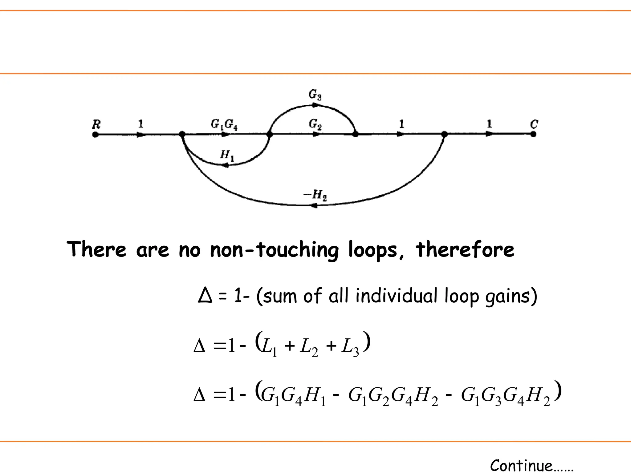
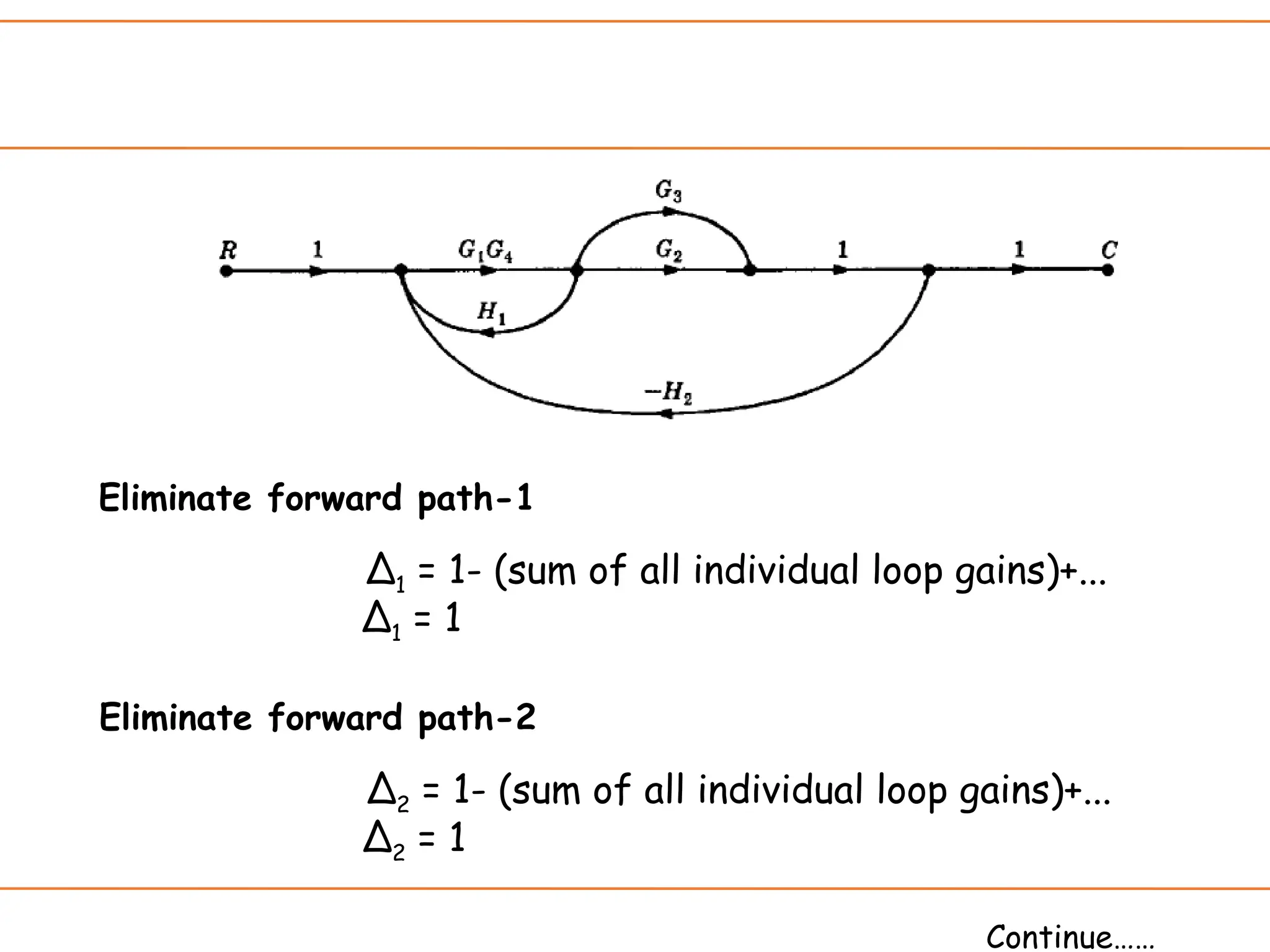
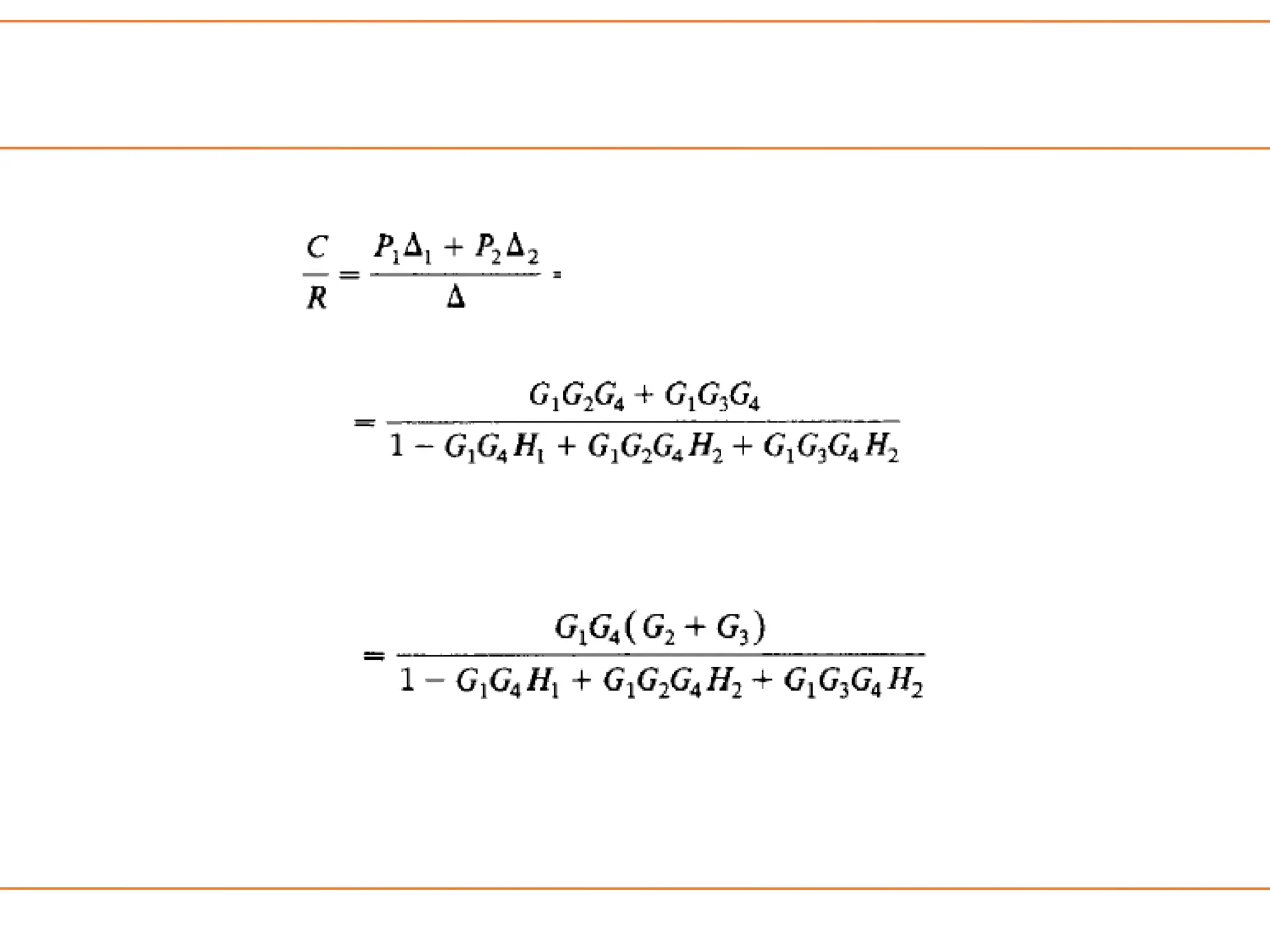
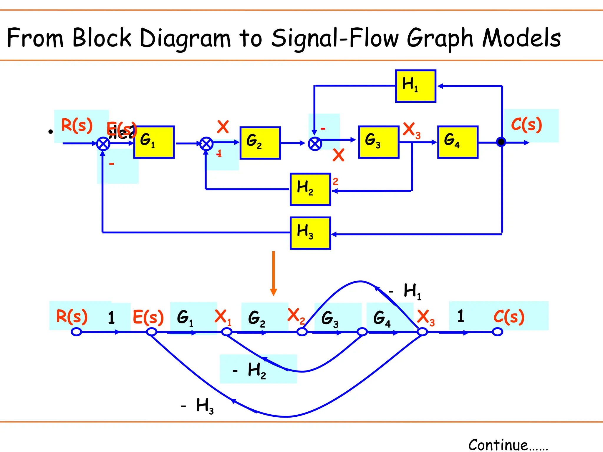
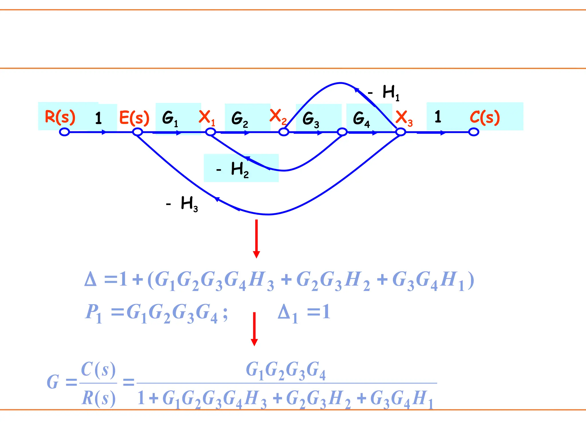
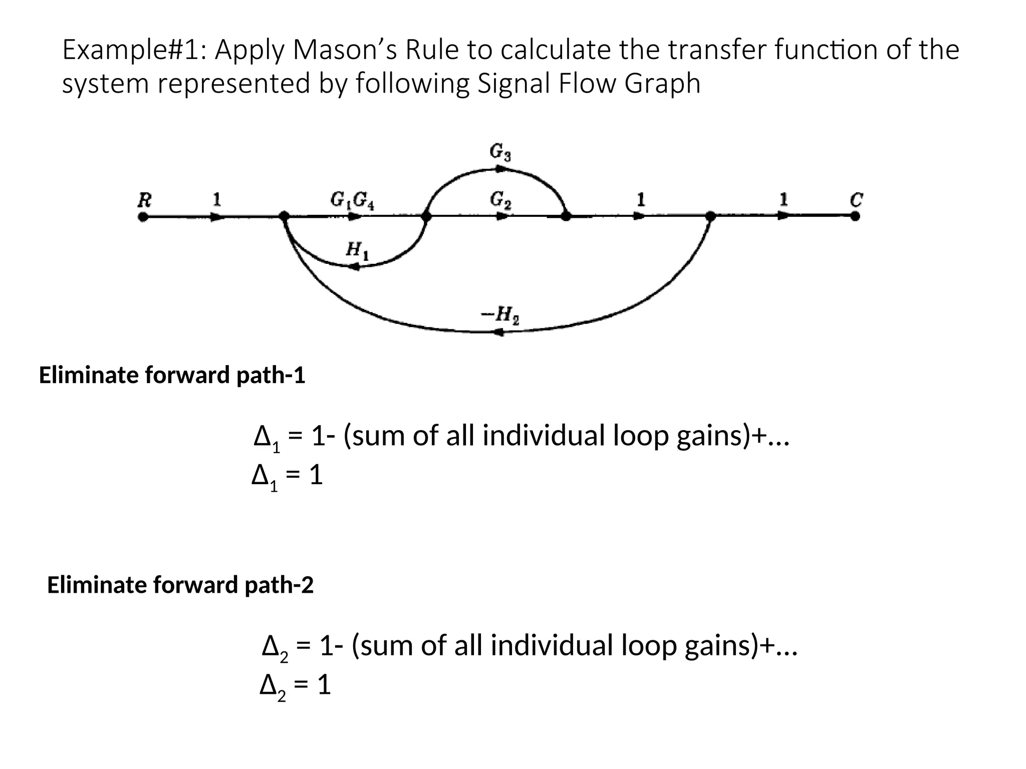
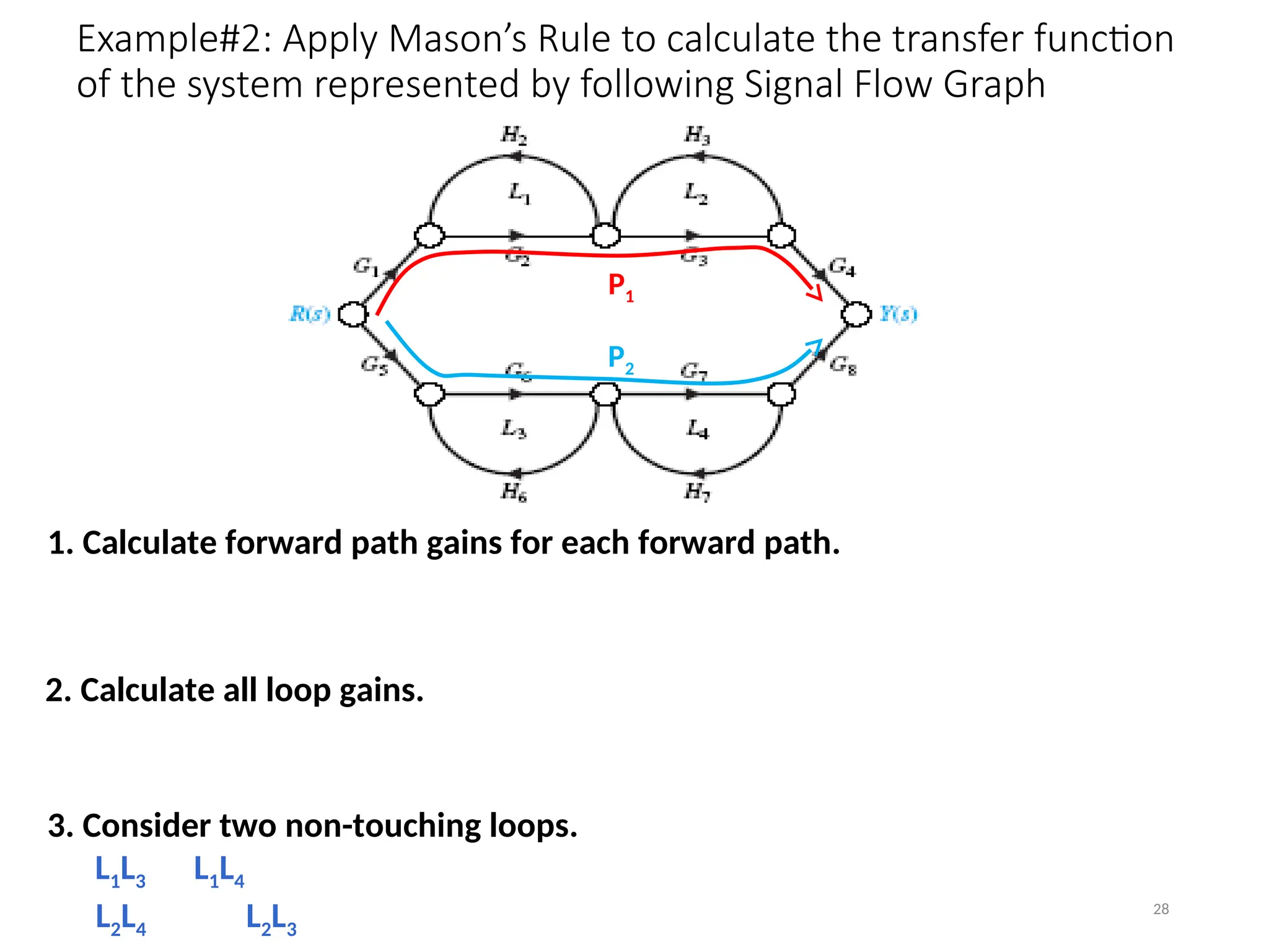
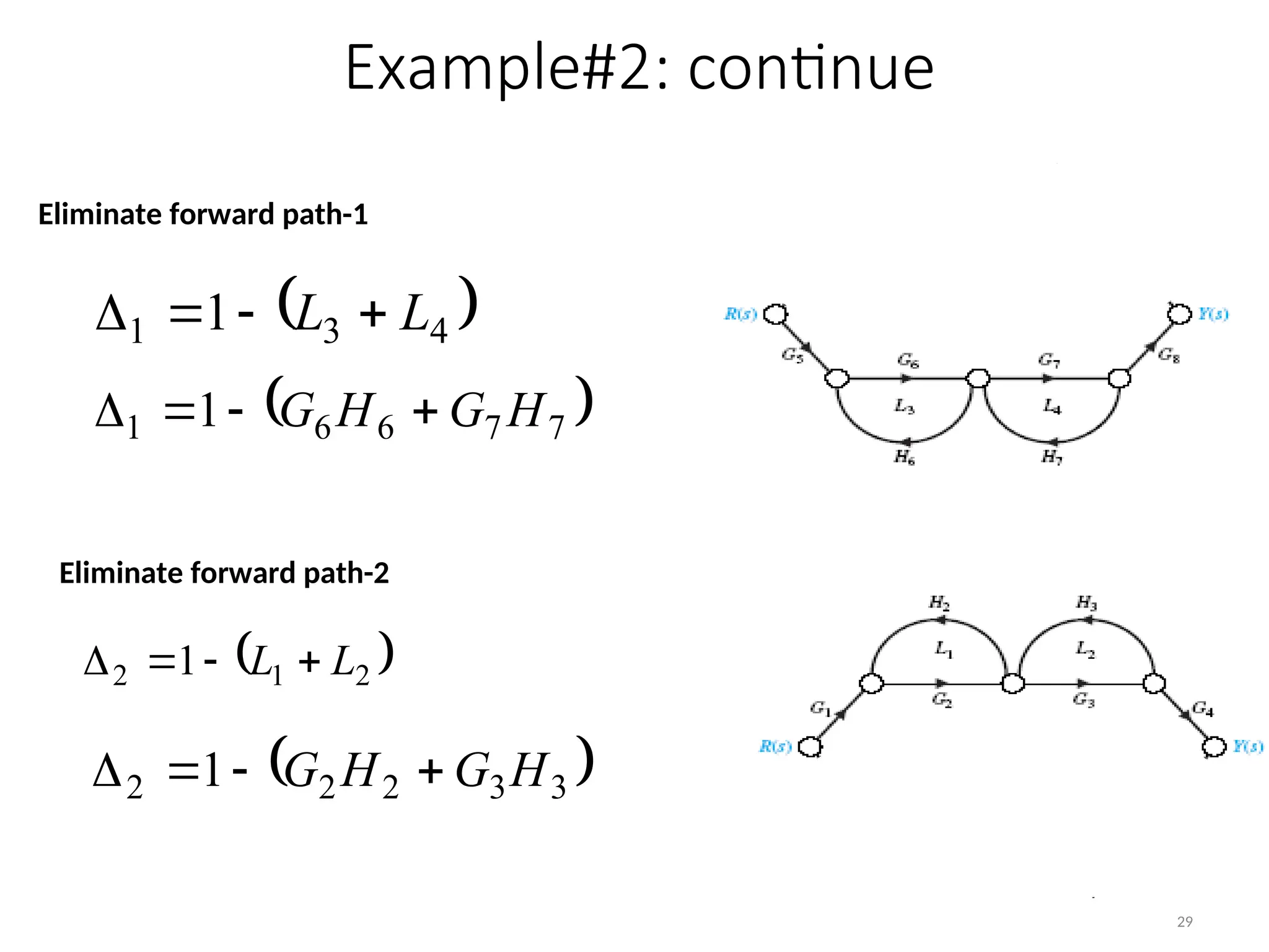
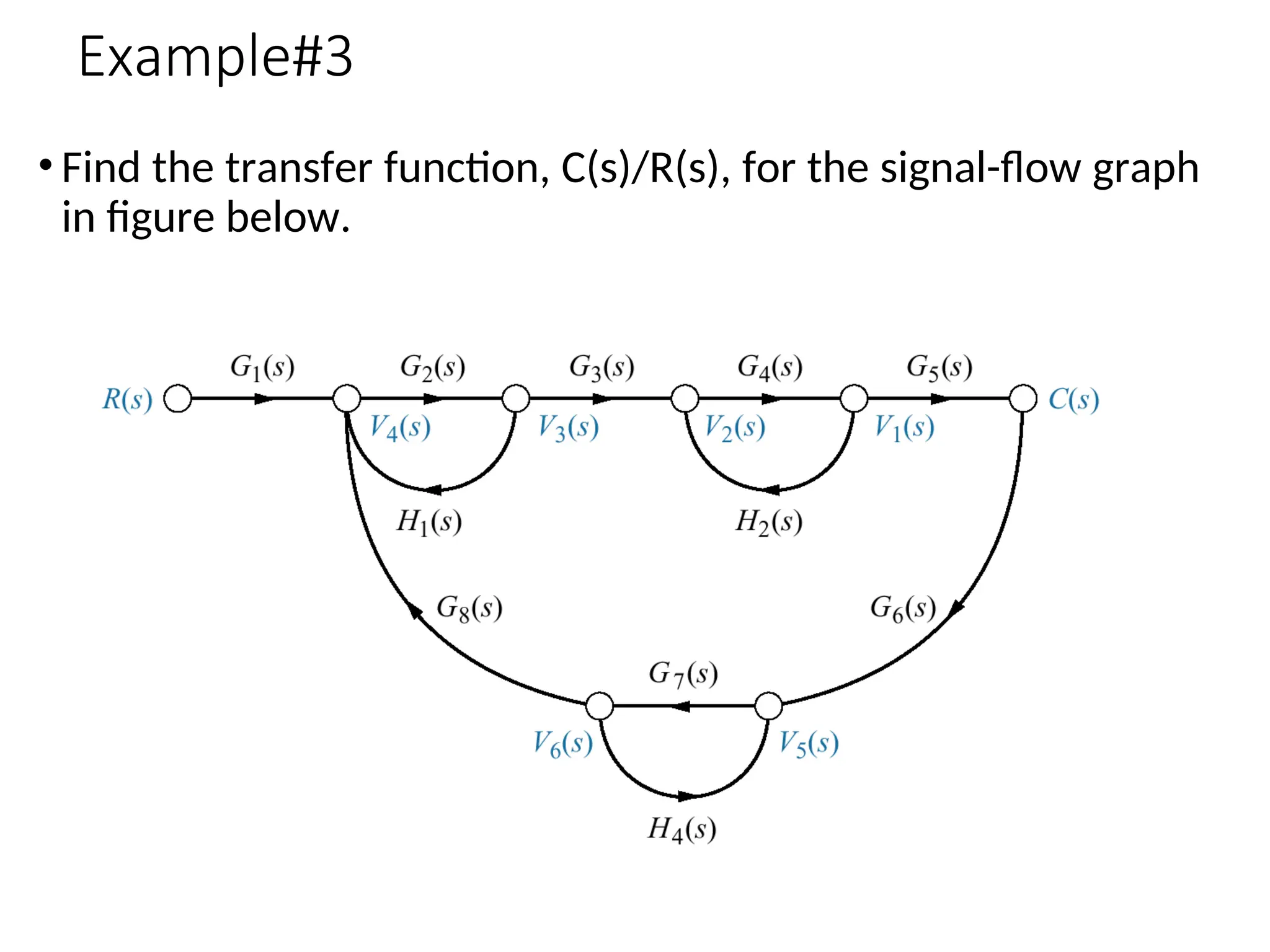
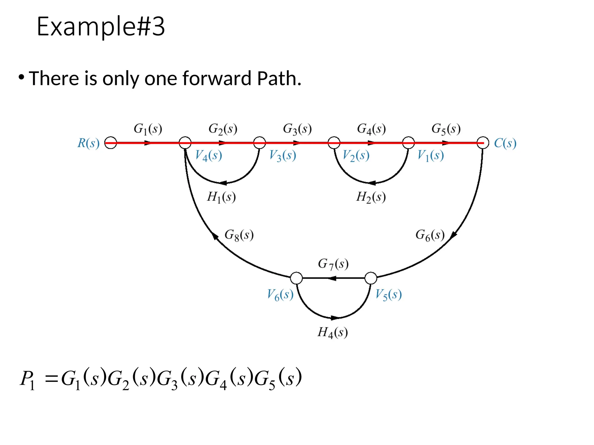
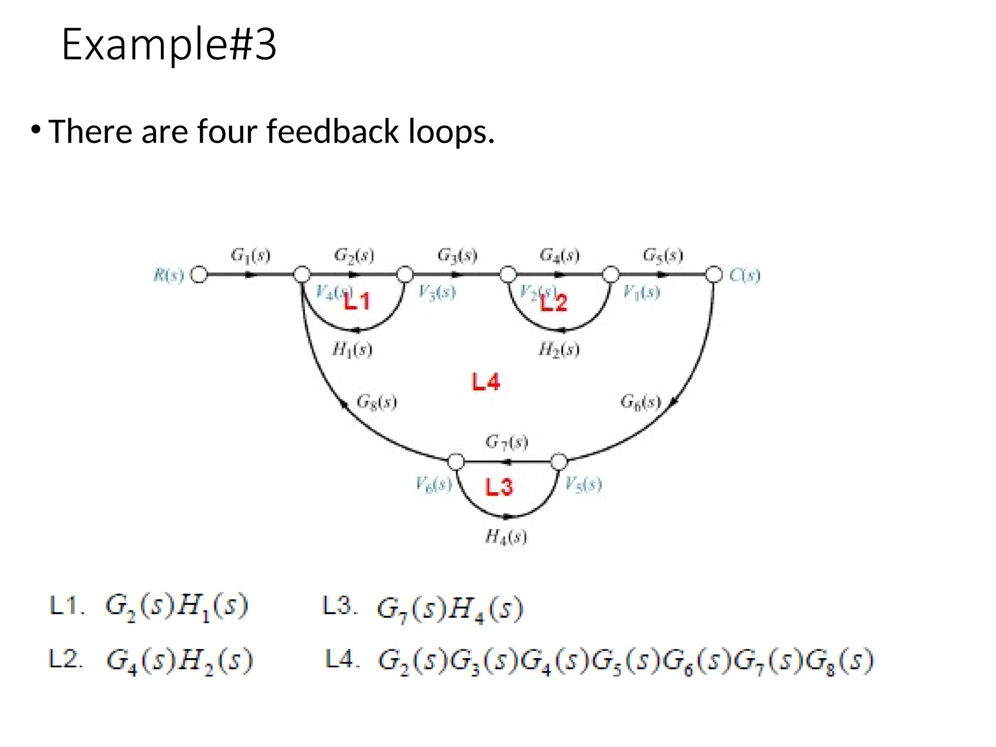
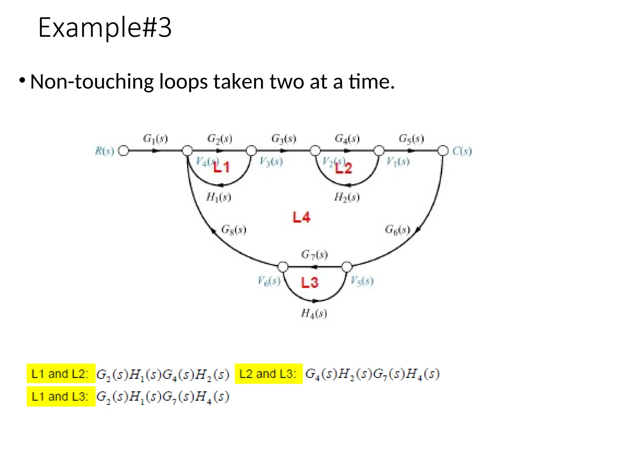
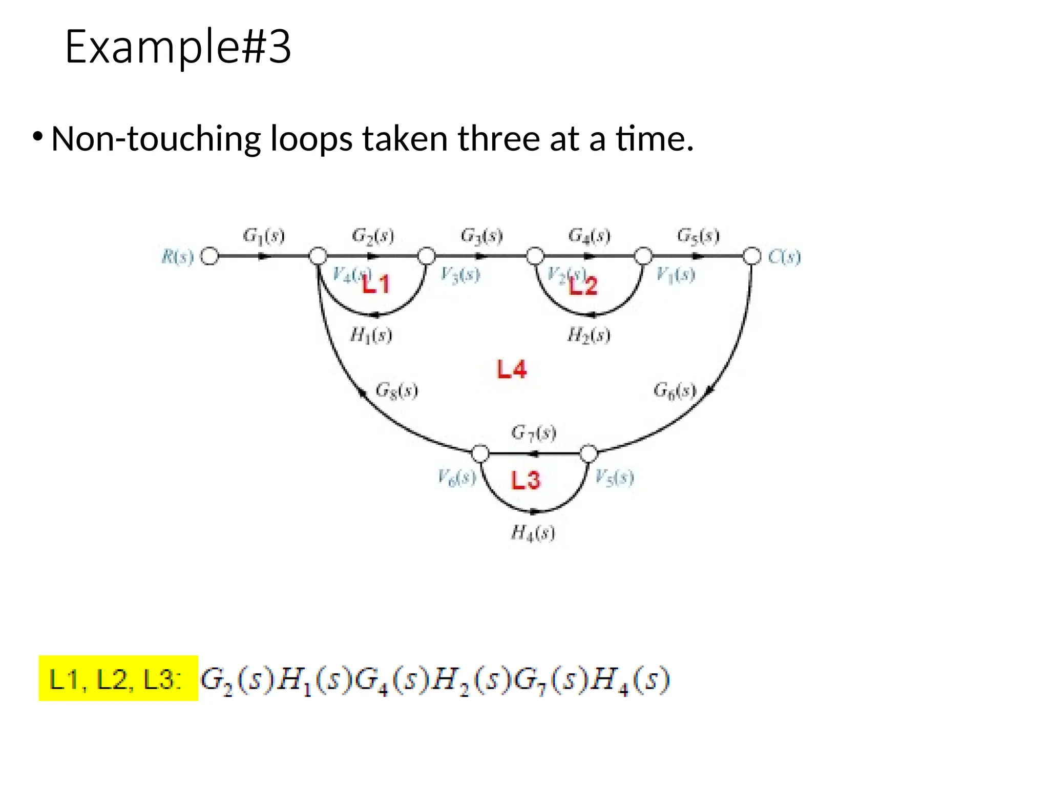
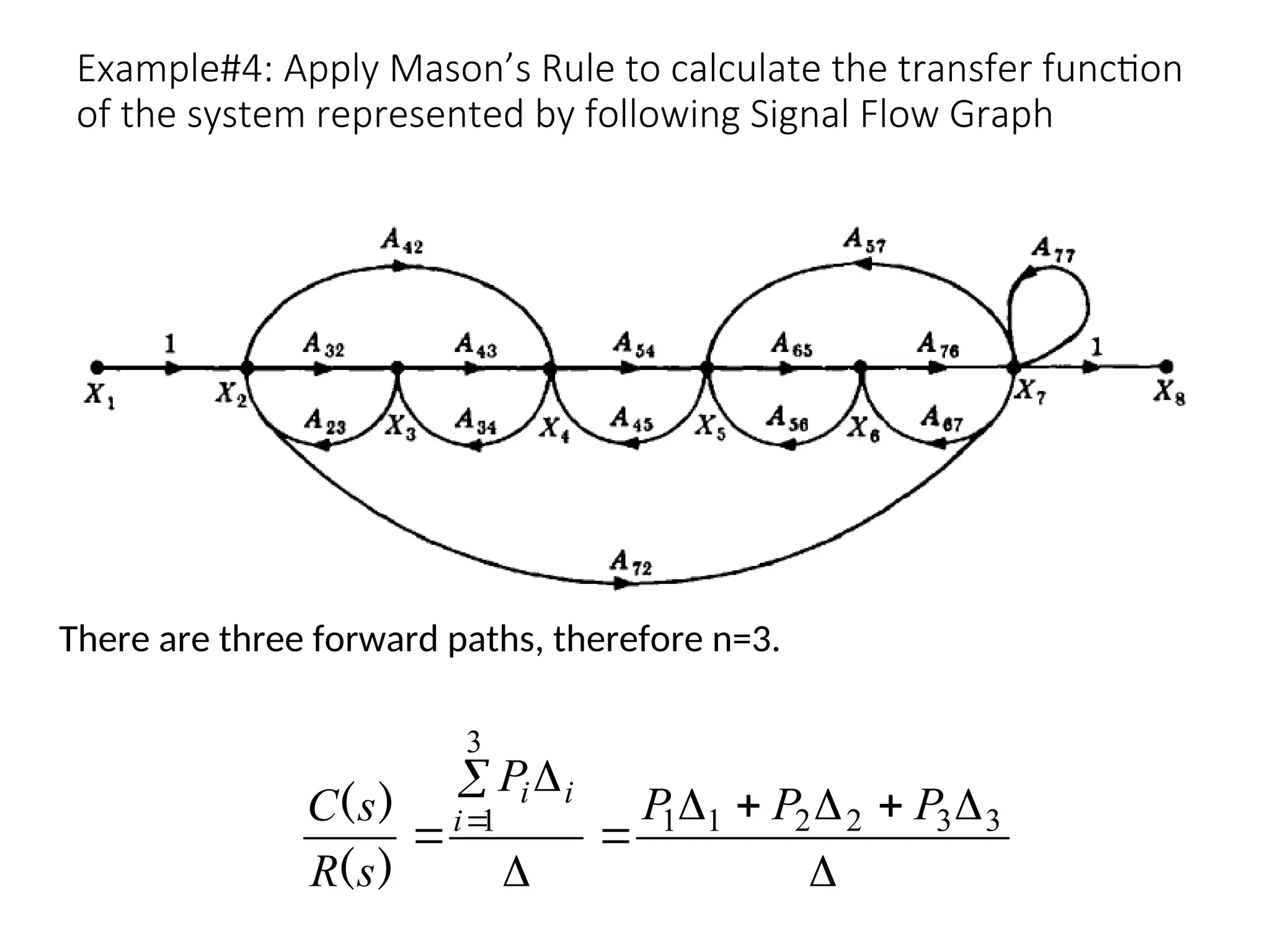
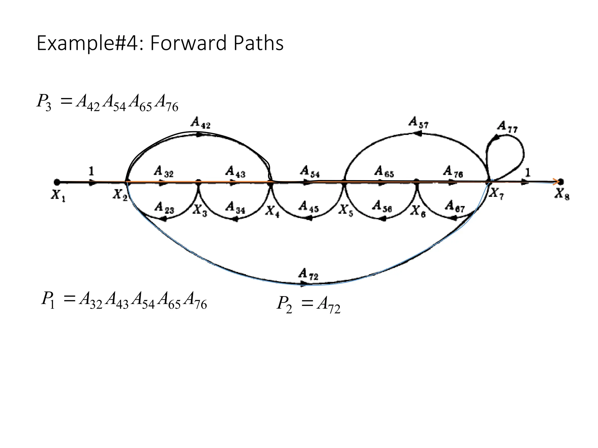
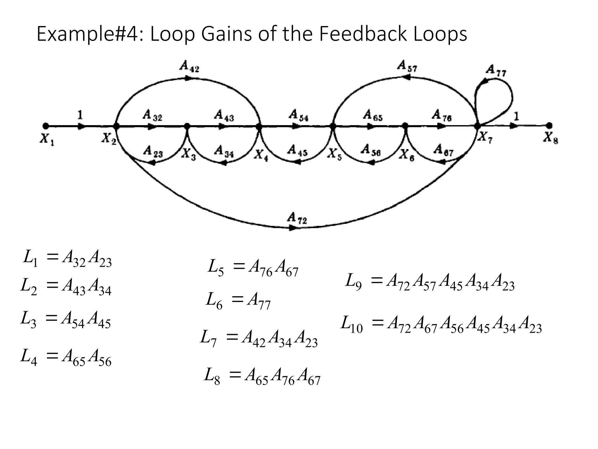
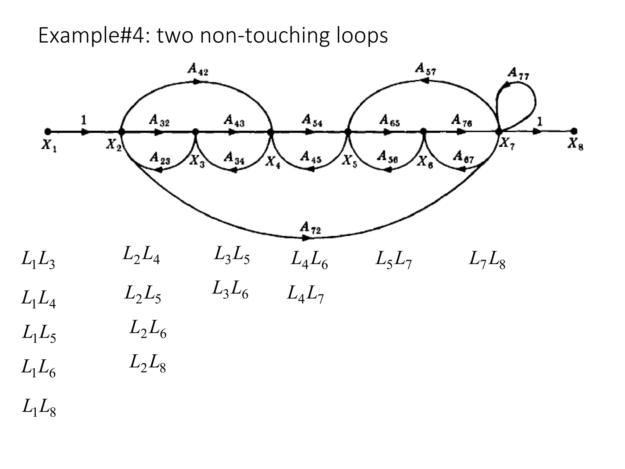
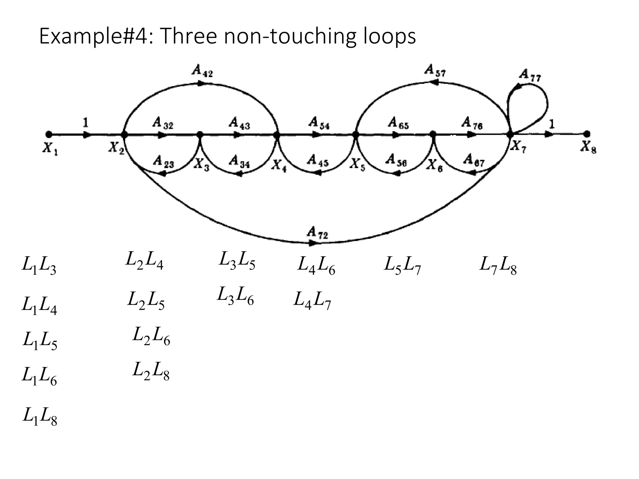
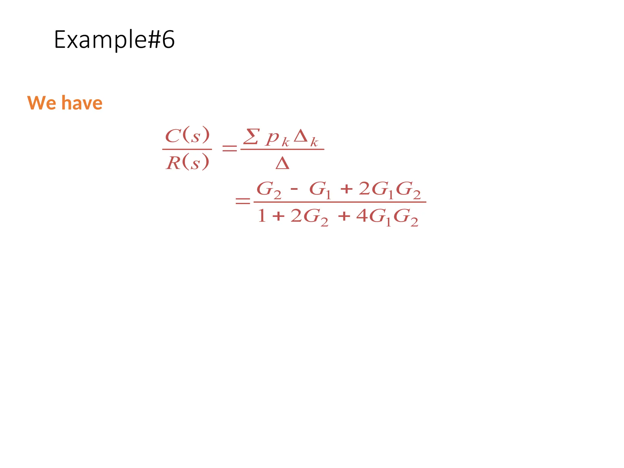
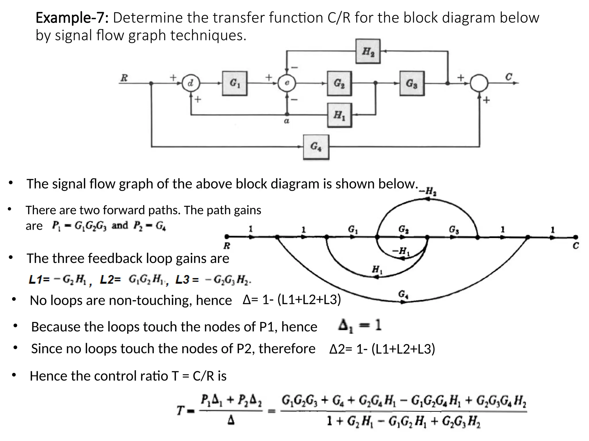
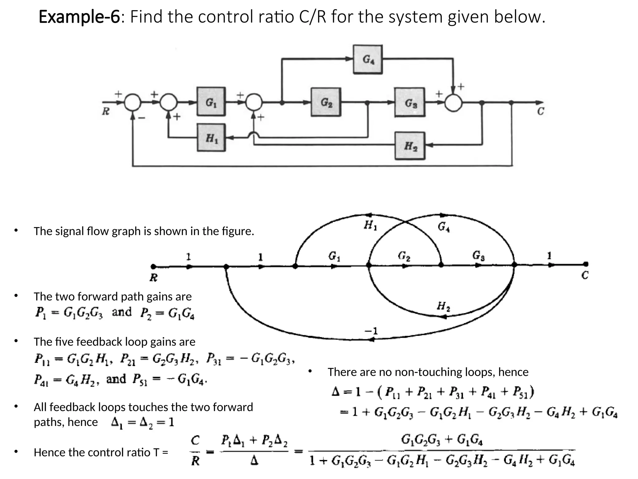
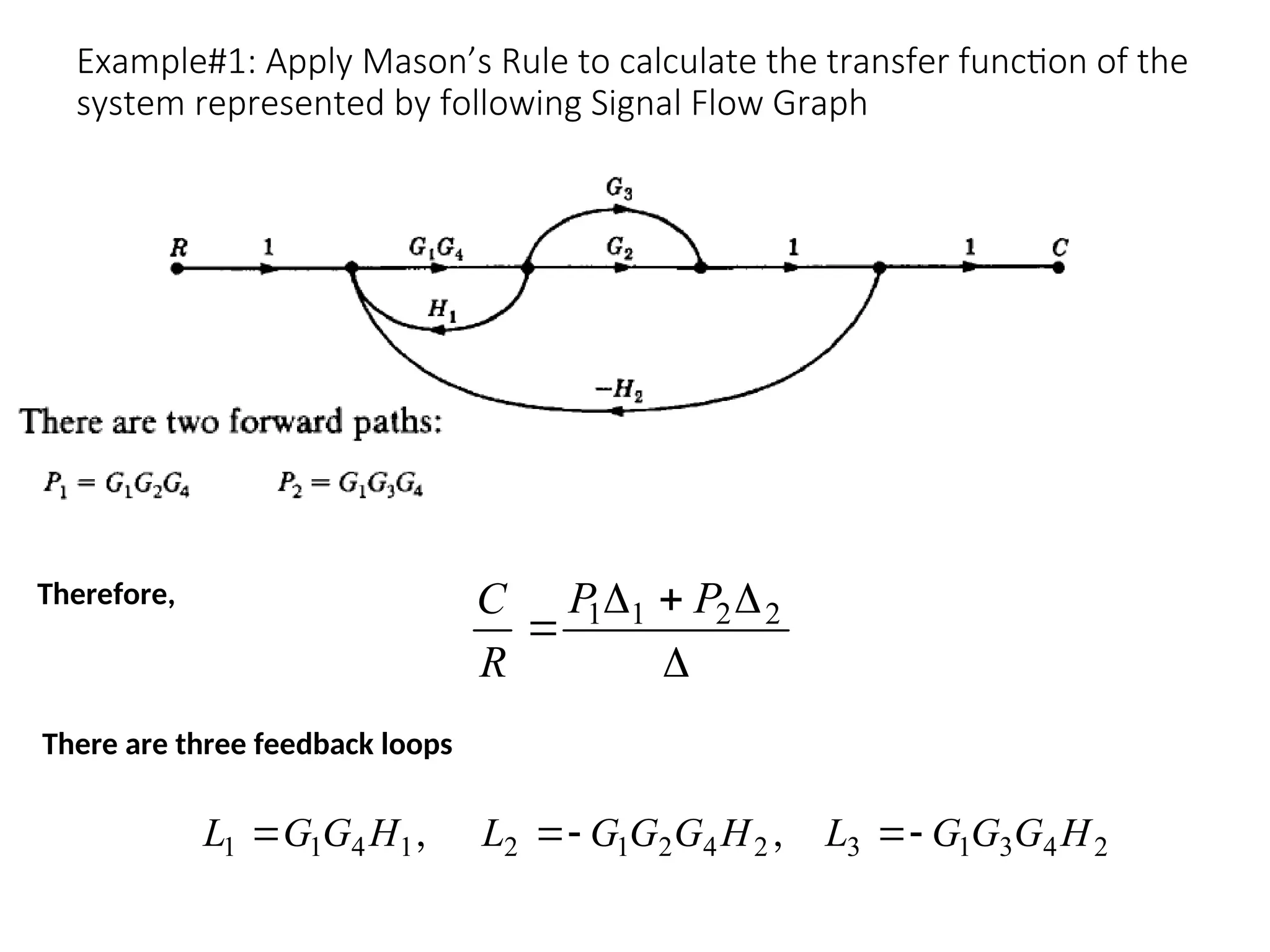
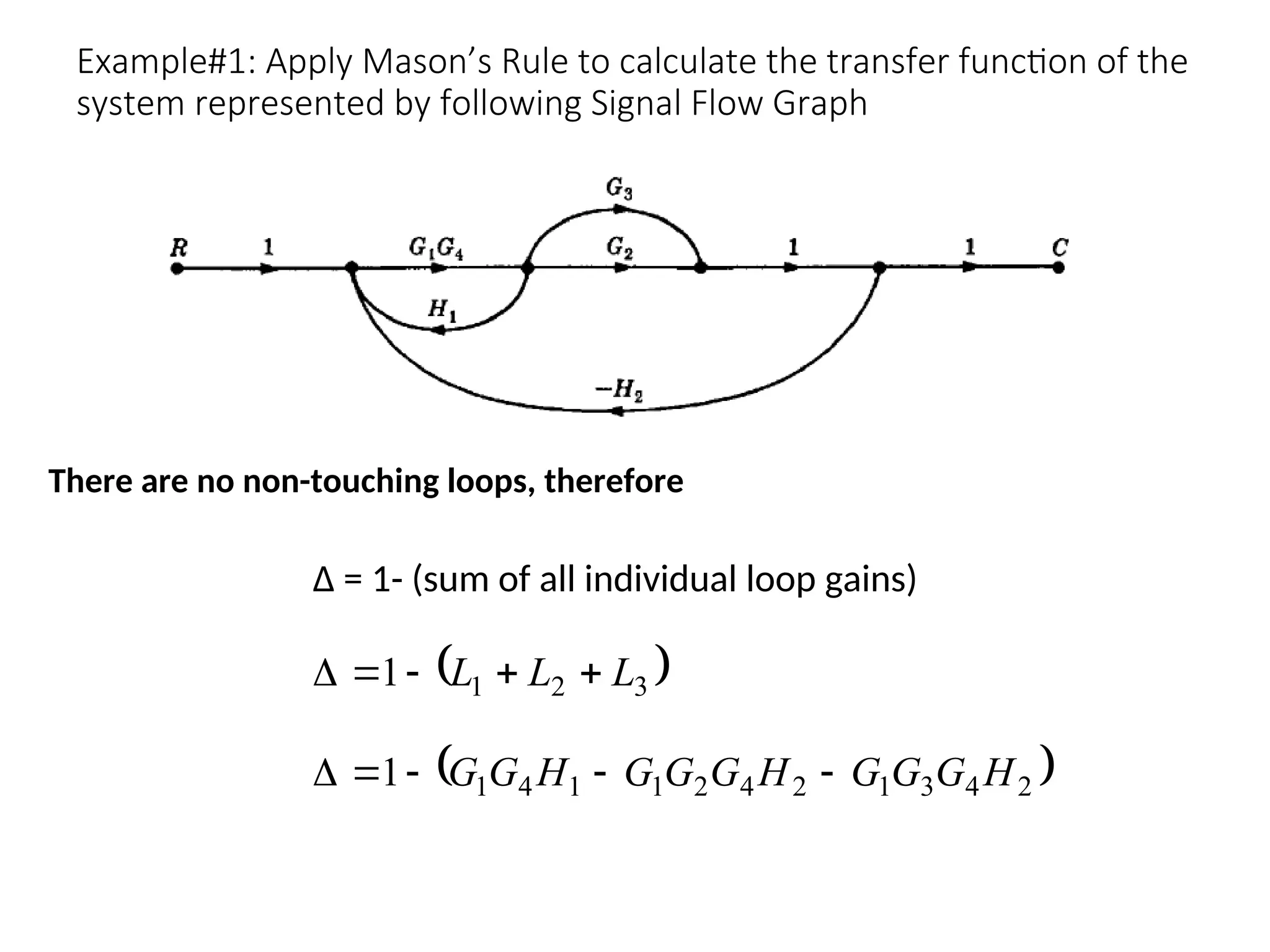
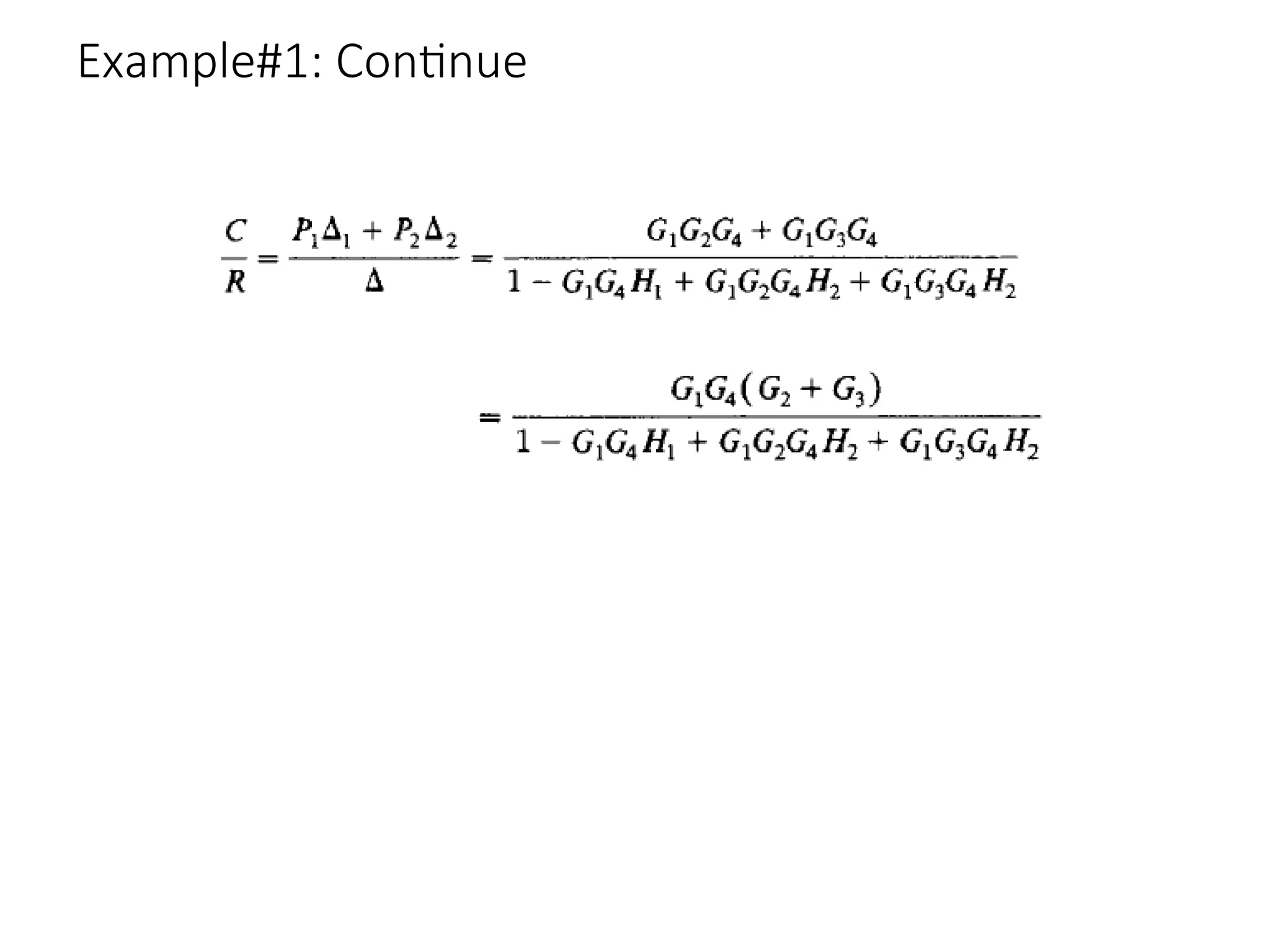
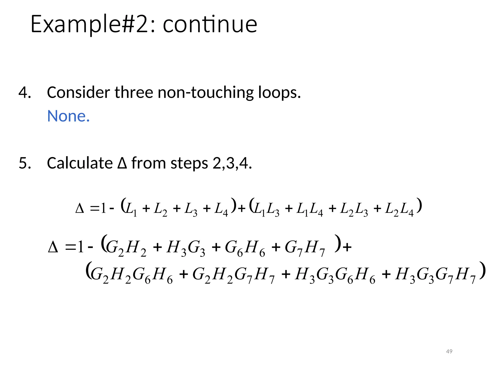
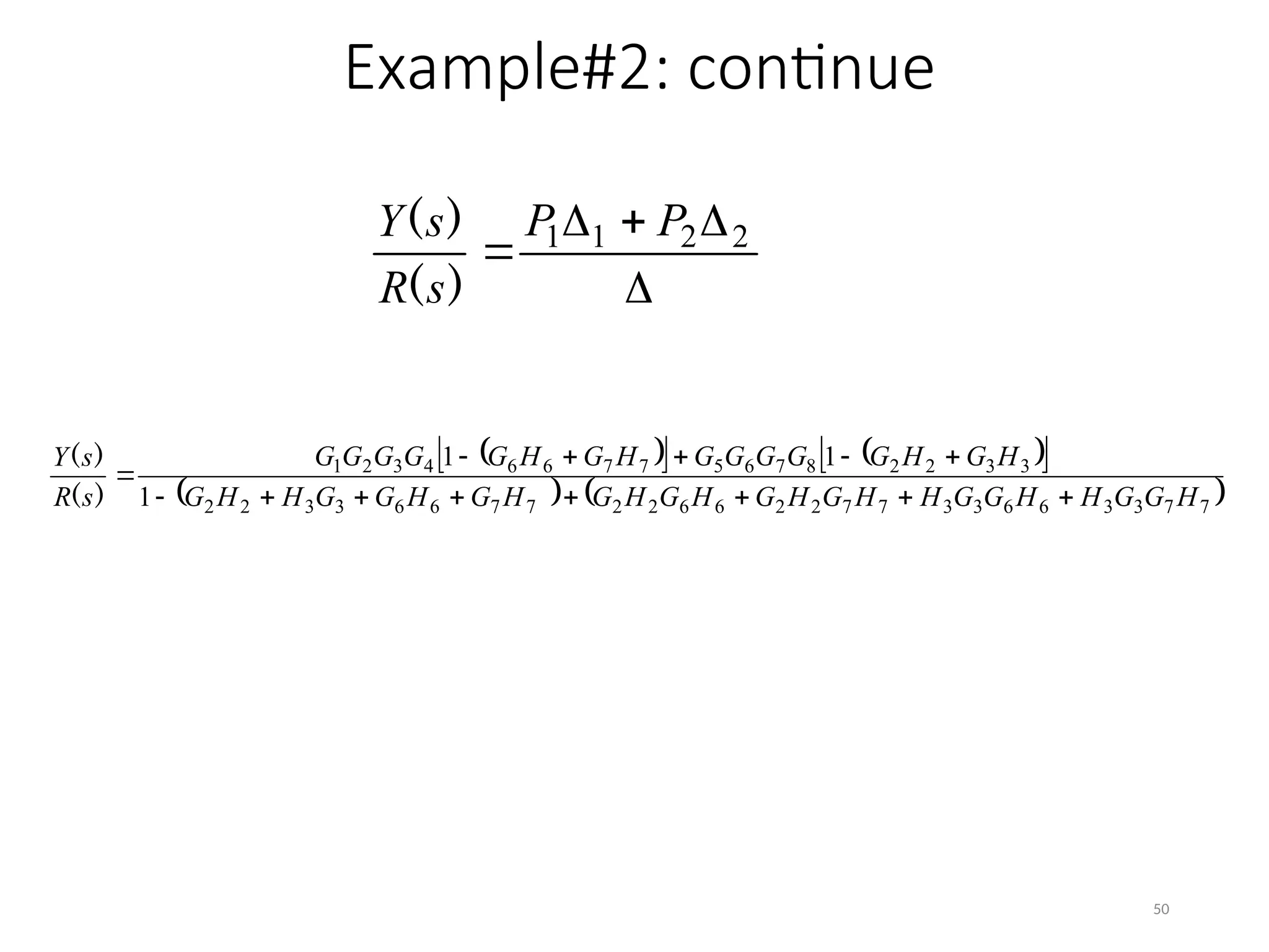
SIGNAL FLOW
GRAPH
CONTROL ENGINEERING FUNDAMENTALS
Eng. Mohammed Qasim Taha
Outline
•Introduction to Signal Flow Graphs
• Definitions
• Terminologies
•Mason’s Gain Formula
• Examples
•Signal Flow Graph from Block Diagrams
•Design Examples
Signal Flow Graph (SFG)
• Alternative method to block diagram
representation, developed by Samuel Jefferson
Mason.
• Advantage: the availability of a flow graph gain
formula, also called Mason’s gain formula.
• A signal-flow graph consists of a network in which
nodes are connected by directed branches.
• It depicts the flow of signals from one point of a
system to another and gives the relationships
among the signals.
Fundamentals of Signal Flow Graphs
ax
y 
x y
a
Consider a simple equation below and draw its signal
flow graph:
The signal flow graph of the equation is shown below;
Important terminology :
• Branches :-
line joining two nodes is called branch.
x y
a
Branch
• Dummy Nodes:-
A branch having one can be added at i/p as well as o/p.
Dummy Nodes
Out put node
Input node
b
x4
x3
x2
x1
x0 h
f
g
e
d
c
a
Input & output node
• Input node:-
It is node that has only outgoing branches.
• Output node:-
It is a node that has incoming branches.
Forward path:-
• Any path from i/p node to o/p node.
Forward path
Loop :-
• A closed path from a node to the same node is called
loop.
Self loop:-
•A feedback loop that contains of only one node is
called self loop.
Self loop
Loop gain:-
The product of all the gains forming a loop
Loop gain = A32 A23
Path & path gain
Path:-
A path is a traversal of connected branches in the
direction of branch arrow.
Path gain:-
The product of all branch gains while going through the
forward path it is called as path gain.
Feedback path or loop :-
• it is a path to o/p node to i/p node.
Touching loops:-
• when the loops are having the common node that the
loops are called touching loops.
Non touching loops:-
• when the loops are not having any common node
between them that are called as non- touching loops.
Non-touching loops for forward paths
Chain Node :-
• it is a node that has incoming as well as outgoing
branches.
Chain node
SFG terms representation
Input node (source)
b
1
x a
2
x
c
4
x
d
1
3
x
3
x
Chain node
Chain node
forward path
path
loop
branch
node
transmittance
input node (source)
Output node
Mason’s Rule (Mason, 1953)
• The block diagram reduction technique requires
successive application of fundamental relationships in
order to arrive at the system transfer function.
• On the other hand, Mason’s rule for reducing a
signal-flow graph to a single transfer function
requires the application of one formula.
• The formula was derived by S. J. Mason when he
related the signal-flow graph to the simultaneous
equations that can be written from the graph.
Mason’s Rule :-
• The transfer function, C(s)/R(s), of a system represented by a
signal-flow graph is;
• Where
• n = number of forward paths.
• Pi = the i th forward-path gain.
• ∆ = Determinant of the system
• ∆i = Determinant of the ith forward path

 
 
n
i
i
i
P
s
R
s
C 1
)
(
)
(

 
 
n
i
i
i
P
s
R
s
C 1
)
(
)
(
∆ is called the signal flow graph determinant or characteristic
function. Since ∆=0 is the system characteristic equation.
∆ = 1- (sum of all individual loop gains) + (sum of the products of
the gains of all possible two loops that do not touch each other) –
(sum of the products of the gains of all possible three loops that
do not touch each other) + … and so forth with sums of higher
number of non-touching loop gains
∆i = value of Δ for the part of the block diagram that does not
touch the i-th forward path (Δi = 1 if there are no non-touching
loops to the i-th path.)
Example1: Apply Mason’s Rule to calculate the transfer function
of the system represented by following Signal Flow Graph




 2
2
1
1 P
P
R
C
Therefore,
2
4
3
1
3
2
4
2
1
2
1
4
1
1 H
G
G
G
L
H
G
G
G
L
H
G
G
L 



 ,
,
There are three feedback loops
Continue……
∆ = 1- (sum of all individual loop gains)
There are no non-touching loops, therefore
 
2
4
3
1
2
4
2
1
1
4
1
1 H
G
G
G
H
G
G
G
H
G
G 




 
3
2
1
1 L
L
L 




Continue……
∆2 = 1- (sum of all individual loop gains)+...
Eliminate forward path-2
∆2 = 1
∆1 = 1- (sum of all individual loop gains)+...
Eliminate forward path-1
∆1 = 1
Continue……
From Block Diagram to Signal-Flow Graph Models
• Example2
-
-
-
C(s)
R(s)
G1 G2
H2
H1
G4
G3
H3
E(s) X
1 X
2
X3
R(s)
- H2
1
G4
G3
G2
G1
1 C(s)
- H1
- H3
X1
X2 X3
E(s)
Continue……
R(s)
- H2
1
G4
G3
G2
G1
1 C(s)
- H1
- H3
X1
X2 X3
E(s)
1
4
3
2
3
2
3
4
3
2
1
4
3
2
1
1
)
(
)
(
H
G
G
H
G
G
H
G
G
G
G
G
G
G
G
s
R
s
C
G





1
;
)
(
1
1
4
3
2
1
1
1
4
3
2
3
2
3
4
3
2
1








G
G
G
G
P
H
G
G
H
G
G
H
G
G
G
G
Example#1: Apply Mason’s Rule to calculate the transfer function of the
system represented by following Signal Flow Graph
∆1 = 1- (sum of all individual loop gains)+...
Eliminate forward path-1
∆1 = 1
∆2 = 1- (sum of all individual loop gains)+...
Eliminate forward path-2
∆2 = 1
28
Example#2: Apply Mason’s Rule to calculate the transfer function
of the system represented by following Signal Flow Graph
2. Calculate all loop gains.
3. Consider two non-touching loops.
L1L3 L1L4
L2L4 L2L3
1. Calculate forward path gains for each forward path.
P1
P2
29
Example#2: continue
Eliminate forward path-1
 
4
3
1 1 L
L 



 
2
1
2 1 L
L 



Eliminate forward path-2
 
7
7
6
6
1 1 H
G
H
G 



 
3
3
2
2
2 1 H
G
H
G 



Example#3
• Find the transfer function, C(s)/R(s), for the signal-flow graph
in figure below.
Example#3
• There is only one forward Path.
)
(
)
(
)
(
)
(
)
( s
G
s
G
s
G
s
G
s
G
P 5
4
3
2
1
1 
Example#3
• There are four feedback loops.
Example#3
• Non-touching loops taken two at a time.
Example#3
• Non-touching loops taken three at a time.
Example#3
Eliminate forward path-1
Example#4: Apply Mason’s Rule to calculate the transfer function
of the system represented by following Signal Flow Graph








 
  3
3
2
2
1
1
3
1 P
P
P
P
s
R
s
C i
i
i
)
(
)
(
There are three forward paths, therefore n=3.
Example#4: Forward Paths
72
2 A
P 
76
65
54
43
32
1 A
A
A
A
A
P 
76
65
54
42
3 A
A
A
A
P 
Example#4: Loop Gains of the Feedback Loops
23
32
1 A
A
L 
34
43
2 A
A
L 
45
54
3 A
A
L 
56
65
4 A
A
L 
67
76
5 A
A
L 
77
6 A
L 
23
34
42
7 A
A
A
L 
67
76
65
8 A
A
A
L 
23
34
45
57
72
9 A
A
A
A
A
L 
23
34
45
56
67
72
10 A
A
A
A
A
A
L 
Example#4: two non-touching loops
3
1L
L
4
1L
L
5
1L
L
6
1L
L
8
1L
L
4
2L
L
5
2L
L
6
2L
L
8
2L
L
5
3L
L
6
3L
L
6
4L
L
7
4L
L
7
5L
L 8
7 L
L
Example#4: Three non-touching loops
3
1L
L
4
1L
L
5
1L
L
6
1L
L
8
1L
L
4
2L
L
5
2L
L
6
2L
L
8
2L
L
5
3L
L
6
3L
L
6
4L
L
7
4L
L
7
5L
L 8
7 L
L
G1 G4
G3
From Block Diagram to Signal-Flow Graph Models
Example#5
-
-
-
C(s)
R(s)
G1 G2
H2
H1
G4
G3
H3
E(s) X1
X2
X3
R(s) C(s)
- H2
- H1
- H3
X1
X2 X3
E(s)
1 G2
1
;
)
(
1
1
4
3
2
1
1
1
4
3
2
3
2
3
4
3
2
1








G
G
G
G
P
H
G
G
H
G
G
H
G
G
G
G
1
4
3
2
3
2
3
4
3
2
1
4
3
2
1
1
)
(
)
(
H
G
G
H
G
G
H
G
G
G
G
G
G
G
G
s
R
s
C
G





R(s)
- H2
1
G4
G3
G2
G1
1 C(s)
- H1
- H3
X1
X2 X3
E(s)
From Block Diagram to Signal-Flow Graph Models
Example#5
Example#6
We have
2
1
2
2
1
1
2
4
2
1
2
G
G
G
G
G
G
G
p
s
R
s
C k
k






 

)
(
)
(
Example-7: Determine the transfer function C/R for the block diagram below
by signal flow graph techniques.
• The signal flow graph of the above block diagram is shown below.
• There are two forward paths. The path gains
are
• The three feedback loop gains are
• No loops are non-touching, hence
• Since no loops touch the nodes of P2, therefore
• Because the loops touch the nodes of P1, hence
• Hence the control ratio T = C/R is
Δ= 1- (L1+L2+L3)
Δ2= 1- (L1+L2+L3)
Example-6: Find the control ratio C/R for the system given below.
• The two forward path gains are
• The signal flow graph is shown in the figure.
• The five feedback loop gains are
• Hence the control ratio T =
• There are no non-touching loops, hence
• All feedback loops touches the two forward
paths, hence
Example#1: Apply Mason’s Rule to calculate the transfer function of the
system represented by following Signal Flow Graph




 2
2
1
1 P
P
R
C
Therefore,
2
4
3
1
3
2
4
2
1
2
1
4
1
1 H
G
G
G
L
H
G
G
G
L
H
G
G
L 



 ,
,
There are three feedback loops
Example#1: Apply Mason’s Rule to calculate the transfer function of the
system represented by following Signal Flow Graph
∆ = 1- (sum of all individual loop gains)
There are no non-touching loops, therefore
 
3
2
1
1 L
L
L 




 
2
4
3
1
2
4
2
1
1
4
1
1 H
G
G
G
H
G
G
G
H
G
G 




Example#1: Continue
4. Consider three non-touching loops.
None.
5. Calculate Δ from steps 2,3,4.
   
4
2
3
2
4
1
3
1
4
3
2
1
1 L
L
L
L
L
L
L
L
L
L
L
L 









49
 
 
7
7
3
3
6
6
3
3
7
7
2
2
6
6
2
2
7
7
6
6
3
3
2
2
1
H
G
G
H
H
G
G
H
H
G
H
G
H
G
H
G
H
G
H
G
G
H
H
G










Example#2: continue




 2
2
1
1 P
P
s
R
s
Y
)
(
)
(
50
Example#2: continue
 
   
 
   
7
7
3
3
6
6
3
3
7
7
2
2
6
6
2
2
7
7
6
6
3
3
2
2
3
3
2
2
8
7
6
5
7
7
6
6
4
3
2
1
1
1
1
H
G
G
H
H
G
G
H
H
G
H
G
H
G
H
G
H
G
H
G
G
H
H
G
H
G
H
G
G
G
G
G
H
G
H
G
G
G
G
G
s
R
s
Y














)
(
)
(

SFG Mason Lecture. Control Systems COURSE ppt

  • 1.
    SIGNAL FLOW GRAPH CONTROL ENGINEERINGFUNDAMENTALS Eng. Mohammed Qasim Taha
  • 2.
    Outline •Introduction to SignalFlow Graphs • Definitions • Terminologies •Mason’s Gain Formula • Examples •Signal Flow Graph from Block Diagrams •Design Examples
  • 3.
    Signal Flow Graph(SFG) • Alternative method to block diagram representation, developed by Samuel Jefferson Mason. • Advantage: the availability of a flow graph gain formula, also called Mason’s gain formula. • A signal-flow graph consists of a network in which nodes are connected by directed branches. • It depicts the flow of signals from one point of a system to another and gives the relationships among the signals.
  • 4.
    Fundamentals of SignalFlow Graphs ax y  x y a Consider a simple equation below and draw its signal flow graph: The signal flow graph of the equation is shown below;
  • 5.
    Important terminology : •Branches :- line joining two nodes is called branch. x y a Branch • Dummy Nodes:- A branch having one can be added at i/p as well as o/p. Dummy Nodes
  • 6.
    Out put node Inputnode b x4 x3 x2 x1 x0 h f g e d c a Input & output node • Input node:- It is node that has only outgoing branches. • Output node:- It is a node that has incoming branches.
  • 7.
    Forward path:- • Anypath from i/p node to o/p node. Forward path
  • 8.
    Loop :- • Aclosed path from a node to the same node is called loop.
  • 9.
    Self loop:- •A feedbackloop that contains of only one node is called self loop. Self loop
  • 10.
    Loop gain:- The productof all the gains forming a loop Loop gain = A32 A23
  • 11.
    Path & pathgain Path:- A path is a traversal of connected branches in the direction of branch arrow. Path gain:- The product of all branch gains while going through the forward path it is called as path gain.
  • 12.
    Feedback path orloop :- • it is a path to o/p node to i/p node.
  • 13.
    Touching loops:- • whenthe loops are having the common node that the loops are called touching loops.
  • 14.
    Non touching loops:- •when the loops are not having any common node between them that are called as non- touching loops.
  • 15.
  • 16.
    Chain Node :- •it is a node that has incoming as well as outgoing branches. Chain node
  • 17.
    SFG terms representation Inputnode (source) b 1 x a 2 x c 4 x d 1 3 x 3 x Chain node Chain node forward path path loop branch node transmittance input node (source) Output node
  • 18.
    Mason’s Rule (Mason,1953) • The block diagram reduction technique requires successive application of fundamental relationships in order to arrive at the system transfer function. • On the other hand, Mason’s rule for reducing a signal-flow graph to a single transfer function requires the application of one formula. • The formula was derived by S. J. Mason when he related the signal-flow graph to the simultaneous equations that can be written from the graph.
  • 19.
    Mason’s Rule :- •The transfer function, C(s)/R(s), of a system represented by a signal-flow graph is; • Where • n = number of forward paths. • Pi = the i th forward-path gain. • ∆ = Determinant of the system • ∆i = Determinant of the ith forward path      n i i i P s R s C 1 ) ( ) (
  • 20.
         n i i i P s R s C1 ) ( ) ( ∆ is called the signal flow graph determinant or characteristic function. Since ∆=0 is the system characteristic equation. ∆ = 1- (sum of all individual loop gains) + (sum of the products of the gains of all possible two loops that do not touch each other) – (sum of the products of the gains of all possible three loops that do not touch each other) + … and so forth with sums of higher number of non-touching loop gains ∆i = value of Δ for the part of the block diagram that does not touch the i-th forward path (Δi = 1 if there are no non-touching loops to the i-th path.)
  • 21.
    Example1: Apply Mason’sRule to calculate the transfer function of the system represented by following Signal Flow Graph      2 2 1 1 P P R C Therefore, 2 4 3 1 3 2 4 2 1 2 1 4 1 1 H G G G L H G G G L H G G L      , , There are three feedback loops Continue……
  • 22.
    ∆ = 1-(sum of all individual loop gains) There are no non-touching loops, therefore   2 4 3 1 2 4 2 1 1 4 1 1 H G G G H G G G H G G        3 2 1 1 L L L      Continue……
  • 23.
    ∆2 = 1-(sum of all individual loop gains)+... Eliminate forward path-2 ∆2 = 1 ∆1 = 1- (sum of all individual loop gains)+... Eliminate forward path-1 ∆1 = 1 Continue……
  • 25.
    From Block Diagramto Signal-Flow Graph Models • Example2 - - - C(s) R(s) G1 G2 H2 H1 G4 G3 H3 E(s) X 1 X 2 X3 R(s) - H2 1 G4 G3 G2 G1 1 C(s) - H1 - H3 X1 X2 X3 E(s) Continue……
  • 26.
    R(s) - H2 1 G4 G3 G2 G1 1 C(s) -H1 - H3 X1 X2 X3 E(s) 1 4 3 2 3 2 3 4 3 2 1 4 3 2 1 1 ) ( ) ( H G G H G G H G G G G G G G G s R s C G      1 ; ) ( 1 1 4 3 2 1 1 1 4 3 2 3 2 3 4 3 2 1         G G G G P H G G H G G H G G G G
  • 27.
    Example#1: Apply Mason’sRule to calculate the transfer function of the system represented by following Signal Flow Graph ∆1 = 1- (sum of all individual loop gains)+... Eliminate forward path-1 ∆1 = 1 ∆2 = 1- (sum of all individual loop gains)+... Eliminate forward path-2 ∆2 = 1
  • 28.
    28 Example#2: Apply Mason’sRule to calculate the transfer function of the system represented by following Signal Flow Graph 2. Calculate all loop gains. 3. Consider two non-touching loops. L1L3 L1L4 L2L4 L2L3 1. Calculate forward path gains for each forward path. P1 P2
  • 29.
    29 Example#2: continue Eliminate forwardpath-1   4 3 1 1 L L       2 1 2 1 L L     Eliminate forward path-2   7 7 6 6 1 1 H G H G       3 3 2 2 2 1 H G H G    
  • 30.
    Example#3 • Find thetransfer function, C(s)/R(s), for the signal-flow graph in figure below.
  • 31.
    Example#3 • There isonly one forward Path. ) ( ) ( ) ( ) ( ) ( s G s G s G s G s G P 5 4 3 2 1 1 
  • 32.
    Example#3 • There arefour feedback loops.
  • 33.
  • 34.
    Example#3 • Non-touching loopstaken three at a time.
  • 35.
  • 36.
    Example#4: Apply Mason’sRule to calculate the transfer function of the system represented by following Signal Flow Graph             3 3 2 2 1 1 3 1 P P P P s R s C i i i ) ( ) ( There are three forward paths, therefore n=3.
  • 37.
    Example#4: Forward Paths 72 2A P  76 65 54 43 32 1 A A A A A P  76 65 54 42 3 A A A A P 
  • 38.
    Example#4: Loop Gainsof the Feedback Loops 23 32 1 A A L  34 43 2 A A L  45 54 3 A A L  56 65 4 A A L  67 76 5 A A L  77 6 A L  23 34 42 7 A A A L  67 76 65 8 A A A L  23 34 45 57 72 9 A A A A A L  23 34 45 56 67 72 10 A A A A A A L 
  • 39.
    Example#4: two non-touchingloops 3 1L L 4 1L L 5 1L L 6 1L L 8 1L L 4 2L L 5 2L L 6 2L L 8 2L L 5 3L L 6 3L L 6 4L L 7 4L L 7 5L L 8 7 L L
  • 40.
    Example#4: Three non-touchingloops 3 1L L 4 1L L 5 1L L 6 1L L 8 1L L 4 2L L 5 2L L 6 2L L 8 2L L 5 3L L 6 3L L 6 4L L 7 4L L 7 5L L 8 7 L L
  • 41.
    G1 G4 G3 From BlockDiagram to Signal-Flow Graph Models Example#5 - - - C(s) R(s) G1 G2 H2 H1 G4 G3 H3 E(s) X1 X2 X3 R(s) C(s) - H2 - H1 - H3 X1 X2 X3 E(s) 1 G2
  • 42.
  • 43.
  • 44.
    Example-7: Determine thetransfer function C/R for the block diagram below by signal flow graph techniques. • The signal flow graph of the above block diagram is shown below. • There are two forward paths. The path gains are • The three feedback loop gains are • No loops are non-touching, hence • Since no loops touch the nodes of P2, therefore • Because the loops touch the nodes of P1, hence • Hence the control ratio T = C/R is Δ= 1- (L1+L2+L3) Δ2= 1- (L1+L2+L3)
  • 45.
    Example-6: Find thecontrol ratio C/R for the system given below. • The two forward path gains are • The signal flow graph is shown in the figure. • The five feedback loop gains are • Hence the control ratio T = • There are no non-touching loops, hence • All feedback loops touches the two forward paths, hence
  • 46.
    Example#1: Apply Mason’sRule to calculate the transfer function of the system represented by following Signal Flow Graph      2 2 1 1 P P R C Therefore, 2 4 3 1 3 2 4 2 1 2 1 4 1 1 H G G G L H G G G L H G G L      , , There are three feedback loops
  • 47.
    Example#1: Apply Mason’sRule to calculate the transfer function of the system represented by following Signal Flow Graph ∆ = 1- (sum of all individual loop gains) There are no non-touching loops, therefore   3 2 1 1 L L L        2 4 3 1 2 4 2 1 1 4 1 1 H G G G H G G G H G G     
  • 48.
  • 49.
    4. Consider threenon-touching loops. None. 5. Calculate Δ from steps 2,3,4.     4 2 3 2 4 1 3 1 4 3 2 1 1 L L L L L L L L L L L L           49     7 7 3 3 6 6 3 3 7 7 2 2 6 6 2 2 7 7 6 6 3 3 2 2 1 H G G H H G G H H G H G H G H G H G H G G H H G           Example#2: continue
  • 50.
         2 2 1 1 P P s R s Y ) ( ) ( 50 Example#2:continue             7 7 3 3 6 6 3 3 7 7 2 2 6 6 2 2 7 7 6 6 3 3 2 2 3 3 2 2 8 7 6 5 7 7 6 6 4 3 2 1 1 1 1 H G G H H G G H H G H G H G H G H G H G G H H G H G H G G G G G H G H G G G G G s R s Y               ) ( ) (