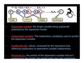
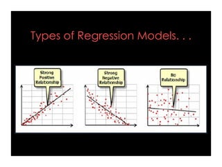
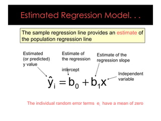
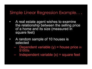
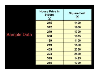
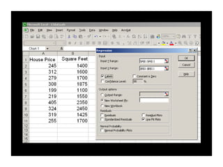
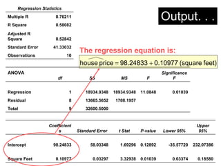
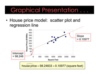
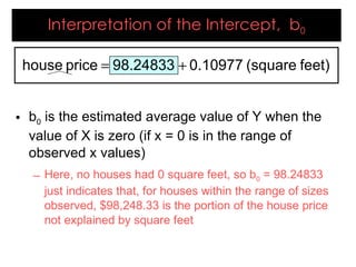
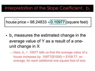
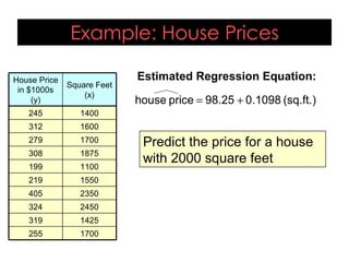
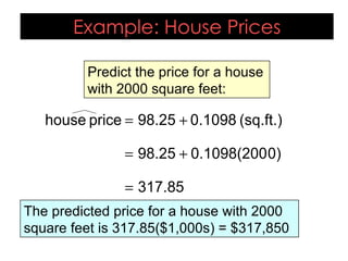
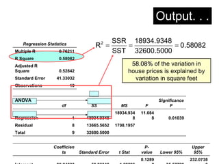
- Regression analysis is a statistical tool used to examine relationships between variables and can help predict future outcomes. It allows one to assess how the value of a dependent variable changes as the value of an independent variable is varied. - Simple linear regression involves one independent variable, while multiple regression can include any number of independent variables. Regression analysis outputs include coefficients, residuals, and measures of fit like the R-squared value. - An example uses home size and price data from 10 houses to generate a linear regression equation predicting that price increases by around $110 for each additional square foot. This model explains 58% of the variation in home prices.

1. REGRESSION ANALYSIS M.Ravishankar [ And it’s application in Business ]

2. Introduction. . . Father of Regression Analysis Carl F. Gauss (1777-1855). contributions to physics, Mathematics & astronomy. The term “Regression” was first used in 1877 by Francis Galton.

3. Regression Analysis. . . It is the study of the relationship between variables. It is one of the most commonly used tools for business analysis. It is easy to use and applies to many situations.

4. Regression types. . . Simple Regression : single explanatory variable Multiple Regression : includes any number of explanatory variables.

5. Dependant variable : the single variable being explained/ predicted by the regression model Independent variable : The explanatory variable(s) used to predict the dependant variable. Coefficients (β): values, computed by the regression tool, reflecting explanatory to dependent variable relationships. Residuals (ε): the portion of the dependent variable that isn ’ t explained by the model; the model under and over predictions.

6. Regression Analysis. . . Linear Regression : straight-line relationship Form: y=mx+b Non-linear : implies curved relationships logarithmic relationships

7. Regression Analysis. . . Cross Sectional : data gathered from the same time period Time Series : Involves data observed over equally spaced points in time.

8. Simple Linear Regression Model. . . Only one independent variable, x Relationship between x and y is described by a linear function Changes in y are assumed to be caused by changes in x

9. Types of Regression Models. . .

10. Estimated Regression Model. . . The sample regression line provides an estimate of the population regression line Estimate of the regression intercept Estimate of the regression slope Estimated (or predicted) y value Independent variable The individual random error terms e i have a mean of zero

11. Simple Linear Regression Example. . . A real estate agent wishes to examine the relationship between the selling price of a home and its size (measured in square feet) A random sample of 10 houses is selected Dependent variable (y) = house price in $1000s Independent variable (x) = square feet

12. Sample Data House Price in $1000s (y) Square Feet (x) 245 1400 312 1600 279 1700 308 1875 199 1100 219 1550 405 2350 324 2450 319 1425 255 1700

14. Output. . . The regression equation is: Regression Statistics Multiple R 0.76211 R Square 0.58082 Adjusted R Square 0.52842 Standard Error 41.33032 Observations 10 ANOVA df SS MS F Significance F Regression 1 18934.9348 18934.9348 11.0848 0.01039 Residual 8 13665.5652 1708.1957 Total 9 32600.5000 Coefficients Standard Error t Stat P-value Lower 95% Upper 95% Intercept 98.24833 58.03348 1.69296 0.12892 -35.57720 232.07386 Square Feet 0.10977 0.03297 3.32938 0.01039 0.03374 0.18580

15. Graphical Presentation . . . House price model: scatter plot and regression line Slope = 0.10977 Intercept = 98.248

16. Interpretation of the Intercept, b 0 b 0 is the estimated average value of Y when the value of X is zero (if x = 0 is in the range of observed x values) Here, no houses had 0 square feet, so b 0 = 98.24833 just indicates that, for houses within the range of sizes observed, $98,248.33 is the portion of the house price not explained by square feet

17. Interpretation of the Slope Coefficient, b 1 b 1 measures the estimated change in the average value of Y as a result of a one-unit change in X Here, b 1 = .10977 tells us that the average value of a house increases by .10977($1000) = $109.77, on average, for each additional one square foot of size

18. Example: House Prices Estimated Regression Equation: Predict the price for a house with 2000 square feet House Price in $1000s (y) Square Feet (x) 245 1400 312 1600 279 1700 308 1875 199 1100 219 1550 405 2350 324 2450 319 1425 255 1700

19. Example: House Prices Predict the price for a house with 2000 square feet: The predicted price for a house with 2000 square feet is 317.85($1,000s) = $317,850

20. Coefficient of determination Coefficient of Determination, R 2 Note: In the single independent variable case, the coefficient of determination is where: R 2 = Coefficient of determination r = Simple correlation coefficient

21. Examples of Approximate R 2 Values R 2 = +1 y x y x R 2 = 1 R 2 = 1 Perfect linear relationship between x and y: 100% of the variation in y is explained by variation in x

22. Examples of Approximate R 2 Values y x y x 0 < R 2 < 1 Weaker linear relationship between x and y: Some but not all of the variation in y is explained by variation in x

23. Examples of Approximate R 2 Values R 2 = 0 No linear relationship between x and y: The value of Y does not depend on x. (None of the variation in y is explained by variation in x) y x R 2 = 0

24. Output. . . 58.08% of the variation in house prices is explained by variation in square feet Regression Statistics Multiple R 0.76211 R Square 0.58082 Adjusted R Square 0.52842 Standard Error 41.33032 Observations 10 ANOVA df SS MS F Significance F Regression 1 18934.9348 18934.9348 11.0848 0.01039 Residual 8 13665.5652 1708.1957 Total 9 32600.5000 Coefficients Standard Error t Stat P-value Lower 95% Upper 95% Intercept 98.24833 58.03348 1.69296 0.12892 -35.57720 232.07386 Square Feet 0.10977 0.03297 3.32938 0.01039 0.03374 0.18580

25. Standard Error of Estimate. . . The standard deviation of the variation of observations around the regression line is estimated by Where SSE = Sum of squares error n = Sample size k = number of independent variables in the model

26. The Standard Deviation of the Regression Slope The standard error of the regression slope coefficient (b 1 ) is estimated by where: = Estimate of the standard error of the least squares slope = Sample standard error of the estimate

27. Output. . . Regression Statistics Multiple R 0.76211 R Square 0.58082 Adjusted R Square 0.52842 Standard Error 41.33032 Observations 10 ANOVA df SS MS F Significance F Regression 1 18934.9348 18934.9348 11.0848 0.01039 Residual 8 13665.5652 1708.1957 Total 9 32600.5000 Coefficients Standard Error t Stat P-value Lower 95% Upper 95% Intercept 98.24833 58.03348 1.69296 0.12892 -35.57720 232.07386 Square Feet 0.10977 0.03297 3.32938 0.01039 0.03374 0.18580

28. Reference. . . Business statistics by S.P.Gupta & M.P.Gupta Sources retrieved from Internet… www.humboldt.edu www.cs.usask.ca www.cab.latech.edu www.quickmba.com www.wikipedia.com www.youtube.com

29. M.RAVISHANKAR MBA(AB) 2008-2010 Batch NIFTTEA KNITWEAR FASHION INSTITUTE TIRUPUR [email_address]