Downloaded 1,090 times


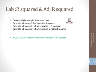


Here are the key steps and results: 1. Load the data and run a multiple linear regression with x1 as the target and x2, x3 as predictors. R-squared is 0.89 2. Add x4, x5 as additional predictors. R-squared increases to 0.94 3. Add x6, x7 as additional predictors. R-squared further increases to 0.98 So as more predictors are added, the R-squared value increases, indicating more of the variation in x1 is explained by the model. However, adding too many predictors can lead to overfitting.