Download as PDF, PPTX


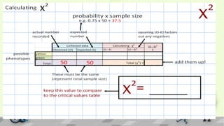


The chi-square distribution is used to test hypotheses about categorical data. It is defined as the sum of the squares of the differences between observed and expected frequencies divided by the expected frequencies. The chi-square distribution depends on the degrees of freedom, with each number of degrees of freedom having a different distribution. The chi-square test can be used to test goodness of fit, independence, and homogeneity. It requires data to be in the form of frequencies in a contingency table and assumes independence between observations.