SlideShare a Scribd company logo
Linear Regression
Simple Linear Regression
Simple linear regression is when you want to
predict values of one variable, given values of
another variable. For example, you might want to
predict a person's height (in inches) from his
weight (in pounds).
Imagine a sample of ten people for whom you know
their height and weight. You could plot the values
on a graph, with weight on the x axis and height on
the y axis.
If there were a perfect linear relationship between
height and weight, then all 10 points on the graph
would fit on a straight line. But, this is never the
case (unless your data are rigged). If there is a
(nonperfect) linear relationship between height and
weight (presumably a positive one), then you would
get a cluster of points on the graph which slopes
upward. In other words, people who weigh a lot
should be taller than those people who are of less
weight. (See graph.)
The purpose of regression analysis is to come up
with an equation of a line that fits through that
cluster of points with the minimal amount of
deviations from the line. The deviation of the
points from the line is called "error." Once you have
this regression equation, if you knew a person's
weight, you could then predict their height. Simple
linear regression is actually the same as a bivariate
correlation between the independent and
dependent variable.
Residuals
After verifying that the linear correlation between two
variables is significant, next we determine the equation of
the line that can be used to predict the value of y for a
given value of x.
Each data point di represents the difference between the
observed y-value and the predicted y-value for a given x-
value on the line. These differences are called residuals.
x
y
d1
d2
d3
For a given x-value,
d = (observed y-value) – (predicted y-value)
Observed
y-value
Predicted
y-value
Regression Line
A regression line, also called a line of best fit, is the line
for which the sum of the squares of the residuals is a
minimum.
The Equation of a Regression Line
The equation of a regression line for an independent variable
x and a dependent variable y is
ŷ = mx + b
where ŷ is the predicted y-value for a given x-value. The
slope m and y-intercept b are given by
  
 
-
-
22
and
where is the mean of the y values and is the mean of the
values. The regression line always passes through ( , ).
n xy x y y xm b y mx m
n nn x x
y x
x x y
     
    
  
Regression Line
Example:
Find the equation of the regression line.
x y xy x2 y2
1 – 3 – 3 1 9
2 – 1 – 2 4 1
3 0 0 9 0
4 1 4 16 1
5 2 10 25 4
15x  1y   9xy  2
55x  2
15y 
  
 22
n xy x y
m
n x x
   

  
  
 2
5(9) 15 1
5(55) 15
 


60
50
 1.2
Continued.
Regression Line
Example continued:
b y mx 
1 15
(1.2)
5 5

  3.8 
The equation of the regression line is
ŷ = 1.2x – 3.8.
2
x
y
1
1
2
3
1 2 3 4 5
 1
( , ) 3,
5
x y 

Regression Line
Example:
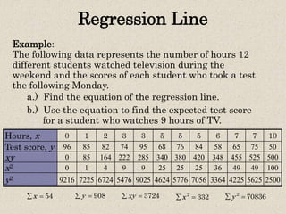
The following data represents the number of hours 12
different students watched television during the
weekend and the scores of each student who took a test
the following Monday.
Hours, x 0 1 2 3 3 5 5 5 6 7 7 10
Test score, y 96 85 82 74 95 68 76 84 58 65 75 50
xy 0 85 164 222 285 340 380 420 348 455 525 500
x2 0 1 4 9 9 25 25 25 36 49 49 100
y2 9216 7225 6724 5476 9025 4624 5776 7056 3364 4225 5625 2500
54x  908y  3724xy  2
332x  2
70836y 
a.) Find the equation of the regression line.
b.) Use the equation to find the expected test score
for a student who watches 9 hours of TV.
Regression Line
Example continued:
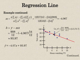
  
 22
n xy x y
m
n x x
   

  
  
 2
12(3724) 54 908
12(332) 54



4.067 
b y mx 
908 54
( 4.067)
12 12
  
93.97
ŷ = –4.07x + 93.97
100
x
y
Hours watching TV
Testscore
80
60
40
20
2 4 6 8 10
   54 908
( , ) , 4.5,75.7
12 12
x y  
Continued.
Regression Line
Example continued:
Using the equation ŷ = –4.07x + 93.97, we can predict
the test score for a student who watches 9 hours of TV.
= –4.07(9) + 93.97
ŷ = –4.07x + 93.97
= 57.34
A student who watches 9 hours of TV over the weekend
can expect to receive about a 57.34 on Monday’s test.
§ 9.3
Measures of
Regression and
Prediction Intervals
Variation About a Regression Line
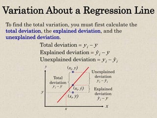
To find the total variation, you must first calculate the
total deviation, the explained deviation, and the
unexplained deviation.
Total deviation iy y 
Explained deviation ˆiy y 
Unexplained deviation ˆi iy y 
x
y (xi, yi)
(xi, ŷi)
(xi, yi)
Unexplained
deviation
ˆi iy y
Total
deviation
iy y
Explained
deviation
ˆiy y
y
x
Variation About a Regression Line
The total variation about a regression line is the sum of the
squares of the differences between the y-value of each ordered
pair and the mean of y.
The explained variation is the sum of the squares of the
differences between each predicted y-value and the mean of y.
The unexplained variation is the sum of the squares of the
differences between the y-value of each ordered pair and each
corresponding predicted y-value.
 2
Total variation iy y  
 2
Explained variation ˆiy y  
 2
Unexplained variation ˆi iy y  
Total variation Explained variation Unexplained variation 
Coefficient of Determination
The coefficient of determination r2 is the ratio of the
explained variation to the total variation. That is,
2 Explained variation
Total variation
r 
Example:
The correlation coefficient for the data that represents
the number of hours students watched television and the
test scores of each student is r  0.831. Find the
coefficient of determination.
2 2
( 0.831)r  
0.691
About 69.1% of the variation in the test
scores can be explained by the variation
in the hours of TV watched. About 30.9%
of the variation is unexplained.
The Standard Error of Estimate
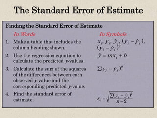
The standard error of estimate se is the standard deviation
of the observed yi -values about the predicted ŷ-value for a
given xi -value. It is given by
where n is the number of ordered pairs in the data set.
2
( )ˆ
2
i i
e
y y
s
n
 


When a ŷ-value is predicted from an x-value, the prediction
is a point estimate.
An interval can also be constructed.
The closer the observed y-values are to the predicted y-values,
the smaller the standard error of estimate will be.
The Standard Error of Estimate
2
, , , ( ),ˆ ˆ
( )ˆ
i i i i i
i i
x y y y y
y y


1. Make a table that includes the
column heading shown.
2. Use the regression equation to
calculate the predicted y-values.
3. Calculate the sum of the squares
of the differences between each
observed y-value and the
corresponding predicted y-value.
4. Find the standard error of
estimate.
Finding the Standard Error of Estimate
In Words In Symbols
ˆ iy mx b 
2
( )ˆi iy y 
2
( )ˆ
2
i i
e
y y
s
n
 


The Standard Error of Estimate
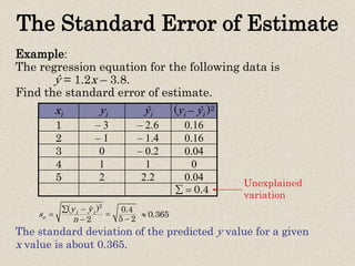
Example:
The regression equation for the following data is
ŷ = 1.2x – 3.8.
Find the standard error of estimate.
xi yi ŷi (yi – ŷi )2
1 – 3 – 2.6 0.16
2 – 1 – 1.4 0.16
3 0 – 0.2 0.04
4 1 1 0
5 2 2.2 0.04
0.4 
Unexplained
variation
2
( )ˆ
2
i i
e
y y
s
n
 


0.4
5 2


0.365
The standard deviation of the predicted y value for a given
x value is about 0.365.
The Standard Error of Estimate
Example:
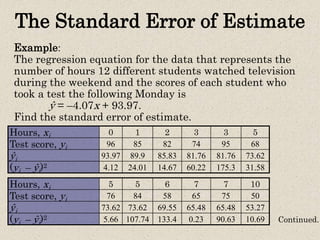
The regression equation for the data that represents the
number of hours 12 different students watched television
during the weekend and the scores of each student who
took a test the following Monday is
ŷ = –4.07x + 93.97.
Find the standard error of estimate.
Hours, xi 0 1 2 3 3 5
Test score, yi 96 85 82 74 95 68
ŷi 93.97 89.9 85.83 81.76 81.76 73.62
(yi – ŷi)2 4.12 24.01 14.67 60.22 175.3 31.58
Hours, xi 5 5 6 7 7 10
Test score, yi 76 84 58 65 75 50
ŷi 73.62 73.62 69.55 65.48 65.48 53.27
(yi – ŷi)2 5.66 107.74 133.4 0.23 90.63 10.69 Continued.
The Standard Error of Estimate
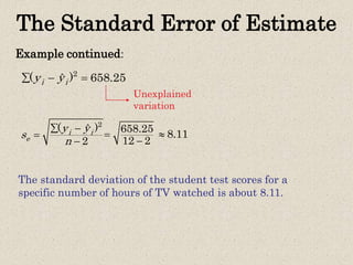
Example continued:
2
( )ˆ
2
i i
e
y y
s
n
 


658.25
12 2


8.11
The standard deviation of the student test scores for a
specific number of hours of TV watched is about 8.11.
2
( ) 658.25ˆi iy y  
Unexplained
variation
Prediction Intervals
Two variables have a bivariate normal distribution if for
any fixed value of x, the corresponding values of y are
normally distributed and for any fixed values of y, the
corresponding x-values are normally distributed.
A prediction interval can be constructed for the true value
of y.
Given a linear regression equation ŷ = mx + b and x0, a
specific value of x, a c-prediction interval for y is
ŷ – E < y < ŷ + E
where
The point estimate is ŷ and the margin of error is E. The
probability that the prediction interval contains y is c.
2
0
2 2
( )1
1 .
( )
c e
n x x
E t s
n n x x

  
  
Prediction Intervals
d.f. 2n 1. Identify the number of ordered
pairs in the data set n and the
degrees of freedom.
2. Use the regression equation and
the given x-value to find the point
estimate ŷ.
3. Find the critical value tc that
corresponds to the given level of
confidence c.
Construct a Prediction Interval for y for a Specific Value of x
In Words In Symbols
ˆ iy mx b 
Use Table 5 in
Appendix B.
Continued.
Prediction Intervals
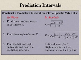
4. Find the standard error
of estimate se.
5. Find the margin of error E.
6. Find the left and right
endpoints and form the
prediction interval.
Construct a Prediction Interval for y for a Specific Value of x
In Words In Symbols
2
( )ˆ
2
i i
e
y y
s
n
 


2
0
2 2
( )1
1
( )
c e
n x x
E t s
n n x x

  
  
Left endpoint: ŷ – E
Right endpoint: ŷ + E
Interval: ŷ – E < y < ŷ + E
Prediction Intervals
Hours, x 0 1 2 3 3 5 5 5 6 7 7 10
Test score, y 96 85 82 74 95 68 76 84 58 65 75 50
Example:
The following data represents the number of hours 12
different students watched television during the
weekend and the scores of each student who took a test
the following Monday.
Continued.
Construct a 95% prediction interval for the test
scores when 4 hours of TV are watched.
ŷ = –4.07x + 93.97 se  8.11
Prediction Intervals
Example continued:
Construct a 95% prediction interval for the test scores
when the number of hours of TV watched is 4.
There are n – 2 = 12 – 2 = 10 degrees of freedom.
ŷ = –4.07x + 93.97= –4.07(4) + 93.97 = 77.69.
The point estimate is
The critical value tc = 2.228, and se = 8.11.
ŷ – E < y < ŷ + E
77.69 – 8.11 = 69.58 77.69+ 8.11 = 85.8
You can be 95% confident that when a student watches 4
hours of TV over the weekend, the student’s test grade will
be between 69.58 and 85.8.
§ 9.4
Multiple Regression
Multiple Regression Equation
In many instances, a better prediction can be found for a
dependent (response) variable by using more than one
independent (explanatory) variable.
For example, a more accurate prediction of Monday’s test grade
from the previous section might be made by considering the
number of other classes a student is taking as well as the
student’s previous knowledge of the test material.
A multiple regression equation has the form
ŷ = b + m1x1 + m2x2 + m3x3 + … + mkxk
where x1, x2, x3,…, xk are independent variables, b is the
y-intercept, and y is the dependent variable.
* Because the mathematics associated with this concept is
complicated, technology is generally used to calculate the multiple
regression equation.
Predicting y-Values
After finding the equation of the multiple regression line, you
can use the equation to predict y-values over the range of the data.
Example:
The following multiple regression equation can be used to predict
the annual U.S. rice yield (in pounds).
ŷ = 859 + 5.76x1 + 3.82x2
where x1 is the number of acres planted (in thousands), and x2 is
the number of acres harvested (in thousands).
(Source: U.S. National Agricultural Statistics Service)
a.) Predict the annual rice yield when x1 = 2758, and x2 = 2714.
b.) Predict the annual rice yield when x1 = 3581, and x2 = 3021.
Continued.
Predicting y-Values
Example continued:
= 859 + 5.76(2758) + 3.82(2714)
= 27,112.56
a.) ŷ = 859 + 5.76x1 + 3.82x2
The predicted annual rice yield is 27,1125.56 pounds.
= 859 + 5.76(3581) + 3.82(3021)
= 33,025.78
b.) ŷ = 859 + 5.76x1 + 3.82x2
The predicted annual rice yield is 33,025.78 pounds.

More Related Content

What's hot

Least Squares Regression Method | Edureka
Least Squares Regression Method | EdurekaLeast Squares Regression Method | Edureka
Least Squares Regression Method | Edureka
Edureka!
 
Regression
RegressionRegression
Regression
LavanyaK75
 
Regression analysis
Regression analysisRegression analysis
Regression analysis
Shameer P Hamsa
 
Linear regression
Linear regressionLinear regression
Linear regression
vermaumeshverma
 
Simple Linear Regression: Step-By-Step
Simple Linear Regression: Step-By-StepSimple Linear Regression: Step-By-Step
Simple Linear Regression: Step-By-Step
Dan Wellisch
 
Presentation On Regression
Presentation On RegressionPresentation On Regression
Presentation On Regression
alok tiwari
 
Regression analysis
Regression analysisRegression analysis
Regression analysisRavi shankar
 
Non Linear Equation
Non Linear EquationNon Linear Equation
Non Linear Equation
MdAlAmin187
 
Simple Linear Regression
Simple Linear RegressionSimple Linear Regression
Simple Linear RegressionSharlaine Ruth
 
Logistic regression
Logistic regressionLogistic regression
Logistic regression
DrZahid Khan
 
Logistic regression
Logistic regressionLogistic regression
Logistic regressionsaba khan
 
An Overview of Simple Linear Regression
An Overview of Simple Linear RegressionAn Overview of Simple Linear Regression
An Overview of Simple Linear Regression
Georgian Court University
 
Regression
Regression Regression
Regression
Ali Raza
 
Basics of Regression analysis
 Basics of Regression analysis Basics of Regression analysis
Basics of Regression analysis
Mahak Vijayvargiya
 
Simple linear regression
Simple linear regressionSimple linear regression
Simple linear regression
Avjinder (Avi) Kaler
 
Lasso and ridge regression
Lasso and ridge regressionLasso and ridge regression
Lasso and ridge regression
SreerajVA
 
Logistic Regression Analysis
Logistic Regression AnalysisLogistic Regression Analysis
Logistic Regression Analysis
COSTARCH Analytical Consulting (P) Ltd.
 
Simple linear regression (final)
Simple linear regression (final)Simple linear regression (final)
Simple linear regression (final)Harsh Upadhyay
 

What's hot (20)

Least Squares Regression Method | Edureka
Least Squares Regression Method | EdurekaLeast Squares Regression Method | Edureka
Least Squares Regression Method | Edureka
 
Regression
RegressionRegression
Regression
 
Regression analysis
Regression analysisRegression analysis
Regression analysis
 
Linear regression
Linear regressionLinear regression
Linear regression
 
Simple Linear Regression: Step-By-Step
Simple Linear Regression: Step-By-StepSimple Linear Regression: Step-By-Step
Simple Linear Regression: Step-By-Step
 
Presentation On Regression
Presentation On RegressionPresentation On Regression
Presentation On Regression
 
Regression analysis
Regression analysisRegression analysis
Regression analysis
 
Regression analysis
Regression analysisRegression analysis
Regression analysis
 
Non Linear Equation
Non Linear EquationNon Linear Equation
Non Linear Equation
 
Simple Linear Regression
Simple Linear RegressionSimple Linear Regression
Simple Linear Regression
 
Logistic regression
Logistic regressionLogistic regression
Logistic regression
 
Logistic regression
Logistic regressionLogistic regression
Logistic regression
 
An Overview of Simple Linear Regression
An Overview of Simple Linear RegressionAn Overview of Simple Linear Regression
An Overview of Simple Linear Regression
 
Regression
Regression Regression
Regression
 
Basics of Regression analysis
 Basics of Regression analysis Basics of Regression analysis
Basics of Regression analysis
 
Simple linear regression
Simple linear regressionSimple linear regression
Simple linear regression
 
Bayes Theorem
Bayes TheoremBayes Theorem
Bayes Theorem
 
Lasso and ridge regression
Lasso and ridge regressionLasso and ridge regression
Lasso and ridge regression
 
Logistic Regression Analysis
Logistic Regression AnalysisLogistic Regression Analysis
Logistic Regression Analysis
 
Simple linear regression (final)
Simple linear regression (final)Simple linear regression (final)
Simple linear regression (final)
 

Similar to Linear regression

Unit3
Unit3Unit3
Bba 3274 qm week 6 part 1 regression models
Bba 3274 qm week 6 part 1 regression modelsBba 3274 qm week 6 part 1 regression models
Bba 3274 qm week 6 part 1 regression models
Stephen Ong
 
Regression
RegressionRegression
Line of best fit lesson
Line of best fit lessonLine of best fit lesson
Line of best fit lesson
ReneeTorres11
 
Regression analysis presentation
Regression analysis presentationRegression analysis presentation
Regression analysis presentation
MuhammadFaisal733
 
Simple linear regression
Simple linear regressionSimple linear regression
Simple linear regressionMaria Theresa
 
Regression analysis by Muthama JM
Regression analysis by Muthama JMRegression analysis by Muthama JM
Regression analysis by Muthama JM
Japheth Muthama
 
Regression Analysis by Muthama JM
Regression Analysis by Muthama JM Regression Analysis by Muthama JM
Regression Analysis by Muthama JM
Japheth Muthama
 
一比一原版(Otago毕业证书)新西兰奥塔哥大学毕业证成绩单
一比一原版(Otago毕业证书)新西兰奥塔哥大学毕业证成绩单一比一原版(Otago毕业证书)新西兰奥塔哥大学毕业证成绩单
一比一原版(Otago毕业证书)新西兰奥塔哥大学毕业证成绩单
ynlsmv4ja
 
一比一原版(RoyalVeterinary毕业证书)皇家兽医学院毕业证成绩单
一比一原版(RoyalVeterinary毕业证书)皇家兽医学院毕业证成绩单一比一原版(RoyalVeterinary毕业证书)皇家兽医学院毕业证成绩单
一比一原版(RoyalVeterinary毕业证书)皇家兽医学院毕业证成绩单
ynlsmv4ja
 
一比一原版(UCD毕业证书)爱尔兰都柏林大学毕业证成绩单
一比一原版(UCD毕业证书)爱尔兰都柏林大学毕业证成绩单一比一原版(UCD毕业证书)爱尔兰都柏林大学毕业证成绩单
一比一原版(UCD毕业证书)爱尔兰都柏林大学毕业证成绩单
ynlsmv4ja
 
一比一原版(UM毕业证书)马来亚大学毕业证成绩单
一比一原版(UM毕业证书)马来亚大学毕业证成绩单一比一原版(UM毕业证书)马来亚大学毕业证成绩单
一比一原版(UM毕业证书)马来亚大学毕业证成绩单
ynlsmv4ja
 
一比一原版(UPM毕业证书)马来西亚博特拉大学毕业证成绩单
一比一原版(UPM毕业证书)马来西亚博特拉大学毕业证成绩单一比一原版(UPM毕业证书)马来西亚博特拉大学毕业证成绩单
一比一原版(UPM毕业证书)马来西亚博特拉大学毕业证成绩单
ynlsmv4ja
 
一比一原版(KHU毕业证书)韩国庆熙大学毕业证成绩单
一比一原版(KHU毕业证书)韩国庆熙大学毕业证成绩单一比一原版(KHU毕业证书)韩国庆熙大学毕业证成绩单
一比一原版(KHU毕业证书)韩国庆熙大学毕业证成绩单
ynlsmv4ja
 
一比一原版(TheAuckland毕业证书)新西兰奥克兰大学毕业证成绩单
一比一原版(TheAuckland毕业证书)新西兰奥克兰大学毕业证成绩单一比一原版(TheAuckland毕业证书)新西兰奥克兰大学毕业证成绩单
一比一原版(TheAuckland毕业证书)新西兰奥克兰大学毕业证成绩单
ynlsmv4ja
 
一比一原版(SEGi毕业证书)马来西亚世纪大学毕业证成绩单
一比一原版(SEGi毕业证书)马来西亚世纪大学毕业证成绩单一比一原版(SEGi毕业证书)马来西亚世纪大学毕业证成绩单
一比一原版(SEGi毕业证书)马来西亚世纪大学毕业证成绩单
ynlsmv4ja
 
Regression analysis: Simple Linear Regression Multiple Linear Regression
Regression analysis:  Simple Linear Regression Multiple Linear RegressionRegression analysis:  Simple Linear Regression Multiple Linear Regression
Regression analysis: Simple Linear Regression Multiple Linear Regression
Ravindra Nath Shukla
 
Descriptive Statistics Formula Sheet Sample Populatio.docx
Descriptive Statistics Formula Sheet    Sample Populatio.docxDescriptive Statistics Formula Sheet    Sample Populatio.docx
Descriptive Statistics Formula Sheet Sample Populatio.docx
simonithomas47935
 
Nonparametric approach to multiple regression
Nonparametric approach to multiple regressionNonparametric approach to multiple regression
Nonparametric approach to multiple regression
Alexander Decker
 
Prac excises 3[1].5
Prac excises 3[1].5Prac excises 3[1].5
Prac excises 3[1].5
Forensic Pathology
 

Similar to Linear regression (20)

Unit3
Unit3Unit3
Unit3
 
Bba 3274 qm week 6 part 1 regression models
Bba 3274 qm week 6 part 1 regression modelsBba 3274 qm week 6 part 1 regression models
Bba 3274 qm week 6 part 1 regression models
 
Regression
RegressionRegression
Regression
 
Line of best fit lesson
Line of best fit lessonLine of best fit lesson
Line of best fit lesson
 
Regression analysis presentation
Regression analysis presentationRegression analysis presentation
Regression analysis presentation
 
Simple linear regression
Simple linear regressionSimple linear regression
Simple linear regression
 
Regression analysis by Muthama JM
Regression analysis by Muthama JMRegression analysis by Muthama JM
Regression analysis by Muthama JM
 
Regression Analysis by Muthama JM
Regression Analysis by Muthama JM Regression Analysis by Muthama JM
Regression Analysis by Muthama JM
 
一比一原版(Otago毕业证书)新西兰奥塔哥大学毕业证成绩单
一比一原版(Otago毕业证书)新西兰奥塔哥大学毕业证成绩单一比一原版(Otago毕业证书)新西兰奥塔哥大学毕业证成绩单
一比一原版(Otago毕业证书)新西兰奥塔哥大学毕业证成绩单
 
一比一原版(RoyalVeterinary毕业证书)皇家兽医学院毕业证成绩单
一比一原版(RoyalVeterinary毕业证书)皇家兽医学院毕业证成绩单一比一原版(RoyalVeterinary毕业证书)皇家兽医学院毕业证成绩单
一比一原版(RoyalVeterinary毕业证书)皇家兽医学院毕业证成绩单
 
一比一原版(UCD毕业证书)爱尔兰都柏林大学毕业证成绩单
一比一原版(UCD毕业证书)爱尔兰都柏林大学毕业证成绩单一比一原版(UCD毕业证书)爱尔兰都柏林大学毕业证成绩单
一比一原版(UCD毕业证书)爱尔兰都柏林大学毕业证成绩单
 
一比一原版(UM毕业证书)马来亚大学毕业证成绩单
一比一原版(UM毕业证书)马来亚大学毕业证成绩单一比一原版(UM毕业证书)马来亚大学毕业证成绩单
一比一原版(UM毕业证书)马来亚大学毕业证成绩单
 
一比一原版(UPM毕业证书)马来西亚博特拉大学毕业证成绩单
一比一原版(UPM毕业证书)马来西亚博特拉大学毕业证成绩单一比一原版(UPM毕业证书)马来西亚博特拉大学毕业证成绩单
一比一原版(UPM毕业证书)马来西亚博特拉大学毕业证成绩单
 
一比一原版(KHU毕业证书)韩国庆熙大学毕业证成绩单
一比一原版(KHU毕业证书)韩国庆熙大学毕业证成绩单一比一原版(KHU毕业证书)韩国庆熙大学毕业证成绩单
一比一原版(KHU毕业证书)韩国庆熙大学毕业证成绩单
 
一比一原版(TheAuckland毕业证书)新西兰奥克兰大学毕业证成绩单
一比一原版(TheAuckland毕业证书)新西兰奥克兰大学毕业证成绩单一比一原版(TheAuckland毕业证书)新西兰奥克兰大学毕业证成绩单
一比一原版(TheAuckland毕业证书)新西兰奥克兰大学毕业证成绩单
 
一比一原版(SEGi毕业证书)马来西亚世纪大学毕业证成绩单
一比一原版(SEGi毕业证书)马来西亚世纪大学毕业证成绩单一比一原版(SEGi毕业证书)马来西亚世纪大学毕业证成绩单
一比一原版(SEGi毕业证书)马来西亚世纪大学毕业证成绩单
 
Regression analysis: Simple Linear Regression Multiple Linear Regression
Regression analysis:  Simple Linear Regression Multiple Linear RegressionRegression analysis:  Simple Linear Regression Multiple Linear Regression
Regression analysis: Simple Linear Regression Multiple Linear Regression
 
Descriptive Statistics Formula Sheet Sample Populatio.docx
Descriptive Statistics Formula Sheet    Sample Populatio.docxDescriptive Statistics Formula Sheet    Sample Populatio.docx
Descriptive Statistics Formula Sheet Sample Populatio.docx
 
Nonparametric approach to multiple regression
Nonparametric approach to multiple regressionNonparametric approach to multiple regression
Nonparametric approach to multiple regression
 
Prac excises 3[1].5
Prac excises 3[1].5Prac excises 3[1].5
Prac excises 3[1].5
 

More from Karishma Chaudhary

Notes on Current trends in IT (1) (1).pdf
Notes on Current trends in IT (1) (1).pdfNotes on Current trends in IT (1) (1).pdf
Notes on Current trends in IT (1) (1).pdf
Karishma Chaudhary
 
Biodiversity 1
Biodiversity 1Biodiversity 1
Biodiversity 1
Karishma Chaudhary
 
History of Operations Research
History of Operations ResearchHistory of Operations Research
History of Operations Research
Karishma Chaudhary
 
Modelling in real world
Modelling in real worldModelling in real world
Modelling in real world
Karishma Chaudhary
 
LPP application and problem formulation
LPP application and problem formulationLPP application and problem formulation
LPP application and problem formulation
Karishma Chaudhary
 
Creativity
Creativity  Creativity
Creativity
Karishma Chaudhary
 
Flair furniture LPP problem
Flair furniture LPP problemFlair furniture LPP problem
Flair furniture LPP problem
Karishma Chaudhary
 
linear programming
linear programminglinear programming
linear programming
Karishma Chaudhary
 
simplex method
simplex methodsimplex method
simplex method
Karishma Chaudhary
 
LPP practice questions
LPP practice questionsLPP practice questions
LPP practice questions
Karishma Chaudhary
 
Technology exports and joint ventures
Technology exports and joint venturesTechnology exports and joint ventures
Technology exports and joint ventures
Karishma Chaudhary
 
Technology management
Technology managementTechnology management
Technology management
Karishma Chaudhary
 
Values, morals and ethics
Values, morals and ethicsValues, morals and ethics
Values, morals and ethics
Karishma Chaudhary
 
Introduction and History of Operations Management
Introduction and History of Operations ManagementIntroduction and History of Operations Management
Introduction and History of Operations Management
Karishma Chaudhary
 
Types of Manufacturing system
Types of Manufacturing systemTypes of Manufacturing system
Types of Manufacturing system
Karishma Chaudhary
 
Over population
Over populationOver population
Over population
Karishma Chaudhary
 
Unemployment in India
Unemployment in IndiaUnemployment in India
Unemployment in India
Karishma Chaudhary
 
Poverty in India
Poverty in IndiaPoverty in India
Poverty in India
Karishma Chaudhary
 
Demographic features of Indian population with recent data
Demographic features of Indian population with recent dataDemographic features of Indian population with recent data
Demographic features of Indian population with recent data
Karishma Chaudhary
 

More from Karishma Chaudhary (20)

Notes on Current trends in IT (1) (1).pdf
Notes on Current trends in IT (1) (1).pdfNotes on Current trends in IT (1) (1).pdf
Notes on Current trends in IT (1) (1).pdf
 
Biodiversity 1
Biodiversity 1Biodiversity 1
Biodiversity 1
 
History of Operations Research
History of Operations ResearchHistory of Operations Research
History of Operations Research
 
Modelling in real world
Modelling in real worldModelling in real world
Modelling in real world
 
LPP application and problem formulation
LPP application and problem formulationLPP application and problem formulation
LPP application and problem formulation
 
Creativity
Creativity  Creativity
Creativity
 
Flair furniture LPP problem
Flair furniture LPP problemFlair furniture LPP problem
Flair furniture LPP problem
 
linear programming
linear programminglinear programming
linear programming
 
Es lecture 1
Es   lecture 1Es   lecture 1
Es lecture 1
 
simplex method
simplex methodsimplex method
simplex method
 
LPP practice questions
LPP practice questionsLPP practice questions
LPP practice questions
 
Technology exports and joint ventures
Technology exports and joint venturesTechnology exports and joint ventures
Technology exports and joint ventures
 
Technology management
Technology managementTechnology management
Technology management
 
Values, morals and ethics
Values, morals and ethicsValues, morals and ethics
Values, morals and ethics
 
Introduction and History of Operations Management
Introduction and History of Operations ManagementIntroduction and History of Operations Management
Introduction and History of Operations Management
 
Types of Manufacturing system
Types of Manufacturing systemTypes of Manufacturing system
Types of Manufacturing system
 
Over population
Over populationOver population
Over population
 
Unemployment in India
Unemployment in IndiaUnemployment in India
Unemployment in India
 
Poverty in India
Poverty in IndiaPoverty in India
Poverty in India
 
Demographic features of Indian population with recent data
Demographic features of Indian population with recent dataDemographic features of Indian population with recent data
Demographic features of Indian population with recent data
 

Recently uploaded

Founder-Game Director Workshop (Session 1)
Founder-Game Director  Workshop (Session 1)Founder-Game Director  Workshop (Session 1)
Founder-Game Director Workshop (Session 1)
Amir H. Fassihi
 
W.H.Bender Quote 65 - The Team Member and Guest Experience
W.H.Bender Quote 65 - The Team Member and Guest ExperienceW.H.Bender Quote 65 - The Team Member and Guest Experience
W.H.Bender Quote 65 - The Team Member and Guest Experience
William (Bill) H. Bender, FCSI
 
Modern Database Management 12th Global Edition by Hoffer solution manual.docx
Modern Database Management 12th Global Edition by Hoffer solution manual.docxModern Database Management 12th Global Edition by Hoffer solution manual.docx
Modern Database Management 12th Global Edition by Hoffer solution manual.docx
ssuserf63bd7
 
Training- integrated management system (iso)
Training- integrated management system (iso)Training- integrated management system (iso)
Training- integrated management system (iso)
akaash13
 
一比一原版杜克大学毕业证(Duke毕业证)成绩单留信认证
一比一原版杜克大学毕业证(Duke毕业证)成绩单留信认证一比一原版杜克大学毕业证(Duke毕业证)成绩单留信认证
一比一原版杜克大学毕业证(Duke毕业证)成绩单留信认证
gcljeuzdu
 
TCS AI for Business Study – Key Findings
TCS AI for Business Study – Key FindingsTCS AI for Business Study – Key Findings
TCS AI for Business Study – Key Findings
Tata Consultancy Services
 
SOCIO-ANTHROPOLOGY FACULTY OF NURSING.....
SOCIO-ANTHROPOLOGY FACULTY OF NURSING.....SOCIO-ANTHROPOLOGY FACULTY OF NURSING.....
SOCIO-ANTHROPOLOGY FACULTY OF NURSING.....
juniourjohnstone
 
Oprah Winfrey: A Leader in Media, Philanthropy, and Empowerment | CIO Women M...
Oprah Winfrey: A Leader in Media, Philanthropy, and Empowerment | CIO Women M...Oprah Winfrey: A Leader in Media, Philanthropy, and Empowerment | CIO Women M...
Oprah Winfrey: A Leader in Media, Philanthropy, and Empowerment | CIO Women M...
CIOWomenMagazine
 
Leadership Ethics and Change, Purpose to Impact Plan
Leadership Ethics and Change, Purpose to Impact PlanLeadership Ethics and Change, Purpose to Impact Plan
Leadership Ethics and Change, Purpose to Impact Plan
Muhammad Adil Jamil
 

Recently uploaded (9)

Founder-Game Director Workshop (Session 1)
Founder-Game Director  Workshop (Session 1)Founder-Game Director  Workshop (Session 1)
Founder-Game Director Workshop (Session 1)
 
W.H.Bender Quote 65 - The Team Member and Guest Experience
W.H.Bender Quote 65 - The Team Member and Guest ExperienceW.H.Bender Quote 65 - The Team Member and Guest Experience
W.H.Bender Quote 65 - The Team Member and Guest Experience
 
Modern Database Management 12th Global Edition by Hoffer solution manual.docx
Modern Database Management 12th Global Edition by Hoffer solution manual.docxModern Database Management 12th Global Edition by Hoffer solution manual.docx
Modern Database Management 12th Global Edition by Hoffer solution manual.docx
 
Training- integrated management system (iso)
Training- integrated management system (iso)Training- integrated management system (iso)
Training- integrated management system (iso)
 
一比一原版杜克大学毕业证(Duke毕业证)成绩单留信认证
一比一原版杜克大学毕业证(Duke毕业证)成绩单留信认证一比一原版杜克大学毕业证(Duke毕业证)成绩单留信认证
一比一原版杜克大学毕业证(Duke毕业证)成绩单留信认证
 
TCS AI for Business Study – Key Findings
TCS AI for Business Study – Key FindingsTCS AI for Business Study – Key Findings
TCS AI for Business Study – Key Findings
 
SOCIO-ANTHROPOLOGY FACULTY OF NURSING.....
SOCIO-ANTHROPOLOGY FACULTY OF NURSING.....SOCIO-ANTHROPOLOGY FACULTY OF NURSING.....
SOCIO-ANTHROPOLOGY FACULTY OF NURSING.....
 
Oprah Winfrey: A Leader in Media, Philanthropy, and Empowerment | CIO Women M...
Oprah Winfrey: A Leader in Media, Philanthropy, and Empowerment | CIO Women M...Oprah Winfrey: A Leader in Media, Philanthropy, and Empowerment | CIO Women M...
Oprah Winfrey: A Leader in Media, Philanthropy, and Empowerment | CIO Women M...
 
Leadership Ethics and Change, Purpose to Impact Plan
Leadership Ethics and Change, Purpose to Impact PlanLeadership Ethics and Change, Purpose to Impact Plan
Leadership Ethics and Change, Purpose to Impact Plan
 

Linear regression

  • 2. Simple Linear Regression Simple linear regression is when you want to predict values of one variable, given values of another variable. For example, you might want to predict a person's height (in inches) from his weight (in pounds). Imagine a sample of ten people for whom you know their height and weight. You could plot the values on a graph, with weight on the x axis and height on the y axis.
  • 3. If there were a perfect linear relationship between height and weight, then all 10 points on the graph would fit on a straight line. But, this is never the case (unless your data are rigged). If there is a (nonperfect) linear relationship between height and weight (presumably a positive one), then you would get a cluster of points on the graph which slopes upward. In other words, people who weigh a lot should be taller than those people who are of less weight. (See graph.)
  • 4.
  • 5. The purpose of regression analysis is to come up with an equation of a line that fits through that cluster of points with the minimal amount of deviations from the line. The deviation of the points from the line is called "error." Once you have this regression equation, if you knew a person's weight, you could then predict their height. Simple linear regression is actually the same as a bivariate correlation between the independent and dependent variable.
  • 6. Residuals After verifying that the linear correlation between two variables is significant, next we determine the equation of the line that can be used to predict the value of y for a given value of x. Each data point di represents the difference between the observed y-value and the predicted y-value for a given x- value on the line. These differences are called residuals. x y d1 d2 d3 For a given x-value, d = (observed y-value) – (predicted y-value) Observed y-value Predicted y-value
  • 7. Regression Line A regression line, also called a line of best fit, is the line for which the sum of the squares of the residuals is a minimum. The Equation of a Regression Line The equation of a regression line for an independent variable x and a dependent variable y is ŷ = mx + b where ŷ is the predicted y-value for a given x-value. The slope m and y-intercept b are given by      - - 22 and where is the mean of the y values and is the mean of the values. The regression line always passes through ( , ). n xy x y y xm b y mx m n nn x x y x x x y              
  • 8. Regression Line Example: Find the equation of the regression line. x y xy x2 y2 1 – 3 – 3 1 9 2 – 1 – 2 4 1 3 0 0 9 0 4 1 4 16 1 5 2 10 25 4 15x  1y   9xy  2 55x  2 15y      22 n xy x y m n x x             2 5(9) 15 1 5(55) 15     60 50  1.2 Continued.
  • 9. Regression Line Example continued: b y mx  1 15 (1.2) 5 5    3.8  The equation of the regression line is ŷ = 1.2x – 3.8. 2 x y 1 1 2 3 1 2 3 4 5  1 ( , ) 3, 5 x y  
  • 10. Regression Line Example: The following data represents the number of hours 12 different students watched television during the weekend and the scores of each student who took a test the following Monday. Hours, x 0 1 2 3 3 5 5 5 6 7 7 10 Test score, y 96 85 82 74 95 68 76 84 58 65 75 50 xy 0 85 164 222 285 340 380 420 348 455 525 500 x2 0 1 4 9 9 25 25 25 36 49 49 100 y2 9216 7225 6724 5476 9025 4624 5776 7056 3364 4225 5625 2500 54x  908y  3724xy  2 332x  2 70836y  a.) Find the equation of the regression line. b.) Use the equation to find the expected test score for a student who watches 9 hours of TV.
  • 11. Regression Line Example continued:     22 n xy x y m n x x             2 12(3724) 54 908 12(332) 54    4.067  b y mx  908 54 ( 4.067) 12 12    93.97 ŷ = –4.07x + 93.97 100 x y Hours watching TV Testscore 80 60 40 20 2 4 6 8 10    54 908 ( , ) , 4.5,75.7 12 12 x y   Continued.
  • 12. Regression Line Example continued: Using the equation ŷ = –4.07x + 93.97, we can predict the test score for a student who watches 9 hours of TV. = –4.07(9) + 93.97 ŷ = –4.07x + 93.97 = 57.34 A student who watches 9 hours of TV over the weekend can expect to receive about a 57.34 on Monday’s test.
  • 13. § 9.3 Measures of Regression and Prediction Intervals
  • 14. Variation About a Regression Line To find the total variation, you must first calculate the total deviation, the explained deviation, and the unexplained deviation. Total deviation iy y  Explained deviation ˆiy y  Unexplained deviation ˆi iy y  x y (xi, yi) (xi, ŷi) (xi, yi) Unexplained deviation ˆi iy y Total deviation iy y Explained deviation ˆiy y y x
  • 15. Variation About a Regression Line The total variation about a regression line is the sum of the squares of the differences between the y-value of each ordered pair and the mean of y. The explained variation is the sum of the squares of the differences between each predicted y-value and the mean of y. The unexplained variation is the sum of the squares of the differences between the y-value of each ordered pair and each corresponding predicted y-value.  2 Total variation iy y    2 Explained variation ˆiy y    2 Unexplained variation ˆi iy y   Total variation Explained variation Unexplained variation 
  • 16. Coefficient of Determination The coefficient of determination r2 is the ratio of the explained variation to the total variation. That is, 2 Explained variation Total variation r  Example: The correlation coefficient for the data that represents the number of hours students watched television and the test scores of each student is r  0.831. Find the coefficient of determination. 2 2 ( 0.831)r   0.691 About 69.1% of the variation in the test scores can be explained by the variation in the hours of TV watched. About 30.9% of the variation is unexplained.
  • 17. The Standard Error of Estimate The standard error of estimate se is the standard deviation of the observed yi -values about the predicted ŷ-value for a given xi -value. It is given by where n is the number of ordered pairs in the data set. 2 ( )ˆ 2 i i e y y s n     When a ŷ-value is predicted from an x-value, the prediction is a point estimate. An interval can also be constructed. The closer the observed y-values are to the predicted y-values, the smaller the standard error of estimate will be.
  • 18. The Standard Error of Estimate 2 , , , ( ),ˆ ˆ ( )ˆ i i i i i i i x y y y y y y   1. Make a table that includes the column heading shown. 2. Use the regression equation to calculate the predicted y-values. 3. Calculate the sum of the squares of the differences between each observed y-value and the corresponding predicted y-value. 4. Find the standard error of estimate. Finding the Standard Error of Estimate In Words In Symbols ˆ iy mx b  2 ( )ˆi iy y  2 ( )ˆ 2 i i e y y s n    
  • 19. The Standard Error of Estimate Example: The regression equation for the following data is ŷ = 1.2x – 3.8. Find the standard error of estimate. xi yi ŷi (yi – ŷi )2 1 – 3 – 2.6 0.16 2 – 1 – 1.4 0.16 3 0 – 0.2 0.04 4 1 1 0 5 2 2.2 0.04 0.4  Unexplained variation 2 ( )ˆ 2 i i e y y s n     0.4 5 2   0.365 The standard deviation of the predicted y value for a given x value is about 0.365.
  • 20. The Standard Error of Estimate Example: The regression equation for the data that represents the number of hours 12 different students watched television during the weekend and the scores of each student who took a test the following Monday is ŷ = –4.07x + 93.97. Find the standard error of estimate. Hours, xi 0 1 2 3 3 5 Test score, yi 96 85 82 74 95 68 ŷi 93.97 89.9 85.83 81.76 81.76 73.62 (yi – ŷi)2 4.12 24.01 14.67 60.22 175.3 31.58 Hours, xi 5 5 6 7 7 10 Test score, yi 76 84 58 65 75 50 ŷi 73.62 73.62 69.55 65.48 65.48 53.27 (yi – ŷi)2 5.66 107.74 133.4 0.23 90.63 10.69 Continued.
  • 21. The Standard Error of Estimate Example continued: 2 ( )ˆ 2 i i e y y s n     658.25 12 2   8.11 The standard deviation of the student test scores for a specific number of hours of TV watched is about 8.11. 2 ( ) 658.25ˆi iy y   Unexplained variation
  • 22. Prediction Intervals Two variables have a bivariate normal distribution if for any fixed value of x, the corresponding values of y are normally distributed and for any fixed values of y, the corresponding x-values are normally distributed. A prediction interval can be constructed for the true value of y. Given a linear regression equation ŷ = mx + b and x0, a specific value of x, a c-prediction interval for y is ŷ – E < y < ŷ + E where The point estimate is ŷ and the margin of error is E. The probability that the prediction interval contains y is c. 2 0 2 2 ( )1 1 . ( ) c e n x x E t s n n x x       
  • 23. Prediction Intervals d.f. 2n 1. Identify the number of ordered pairs in the data set n and the degrees of freedom. 2. Use the regression equation and the given x-value to find the point estimate ŷ. 3. Find the critical value tc that corresponds to the given level of confidence c. Construct a Prediction Interval for y for a Specific Value of x In Words In Symbols ˆ iy mx b  Use Table 5 in Appendix B. Continued.
  • 24. Prediction Intervals 4. Find the standard error of estimate se. 5. Find the margin of error E. 6. Find the left and right endpoints and form the prediction interval. Construct a Prediction Interval for y for a Specific Value of x In Words In Symbols 2 ( )ˆ 2 i i e y y s n     2 0 2 2 ( )1 1 ( ) c e n x x E t s n n x x        Left endpoint: ŷ – E Right endpoint: ŷ + E Interval: ŷ – E < y < ŷ + E
  • 25. Prediction Intervals Hours, x 0 1 2 3 3 5 5 5 6 7 7 10 Test score, y 96 85 82 74 95 68 76 84 58 65 75 50 Example: The following data represents the number of hours 12 different students watched television during the weekend and the scores of each student who took a test the following Monday. Continued. Construct a 95% prediction interval for the test scores when 4 hours of TV are watched. ŷ = –4.07x + 93.97 se  8.11
  • 26. Prediction Intervals Example continued: Construct a 95% prediction interval for the test scores when the number of hours of TV watched is 4. There are n – 2 = 12 – 2 = 10 degrees of freedom. ŷ = –4.07x + 93.97= –4.07(4) + 93.97 = 77.69. The point estimate is The critical value tc = 2.228, and se = 8.11. ŷ – E < y < ŷ + E 77.69 – 8.11 = 69.58 77.69+ 8.11 = 85.8 You can be 95% confident that when a student watches 4 hours of TV over the weekend, the student’s test grade will be between 69.58 and 85.8.
  • 28. Multiple Regression Equation In many instances, a better prediction can be found for a dependent (response) variable by using more than one independent (explanatory) variable. For example, a more accurate prediction of Monday’s test grade from the previous section might be made by considering the number of other classes a student is taking as well as the student’s previous knowledge of the test material. A multiple regression equation has the form ŷ = b + m1x1 + m2x2 + m3x3 + … + mkxk where x1, x2, x3,…, xk are independent variables, b is the y-intercept, and y is the dependent variable. * Because the mathematics associated with this concept is complicated, technology is generally used to calculate the multiple regression equation.
  • 29. Predicting y-Values After finding the equation of the multiple regression line, you can use the equation to predict y-values over the range of the data. Example: The following multiple regression equation can be used to predict the annual U.S. rice yield (in pounds). ŷ = 859 + 5.76x1 + 3.82x2 where x1 is the number of acres planted (in thousands), and x2 is the number of acres harvested (in thousands). (Source: U.S. National Agricultural Statistics Service) a.) Predict the annual rice yield when x1 = 2758, and x2 = 2714. b.) Predict the annual rice yield when x1 = 3581, and x2 = 3021. Continued.
  • 30. Predicting y-Values Example continued: = 859 + 5.76(2758) + 3.82(2714) = 27,112.56 a.) ŷ = 859 + 5.76x1 + 3.82x2 The predicted annual rice yield is 27,1125.56 pounds. = 859 + 5.76(3581) + 3.82(3021) = 33,025.78 b.) ŷ = 859 + 5.76x1 + 3.82x2 The predicted annual rice yield is 33,025.78 pounds.