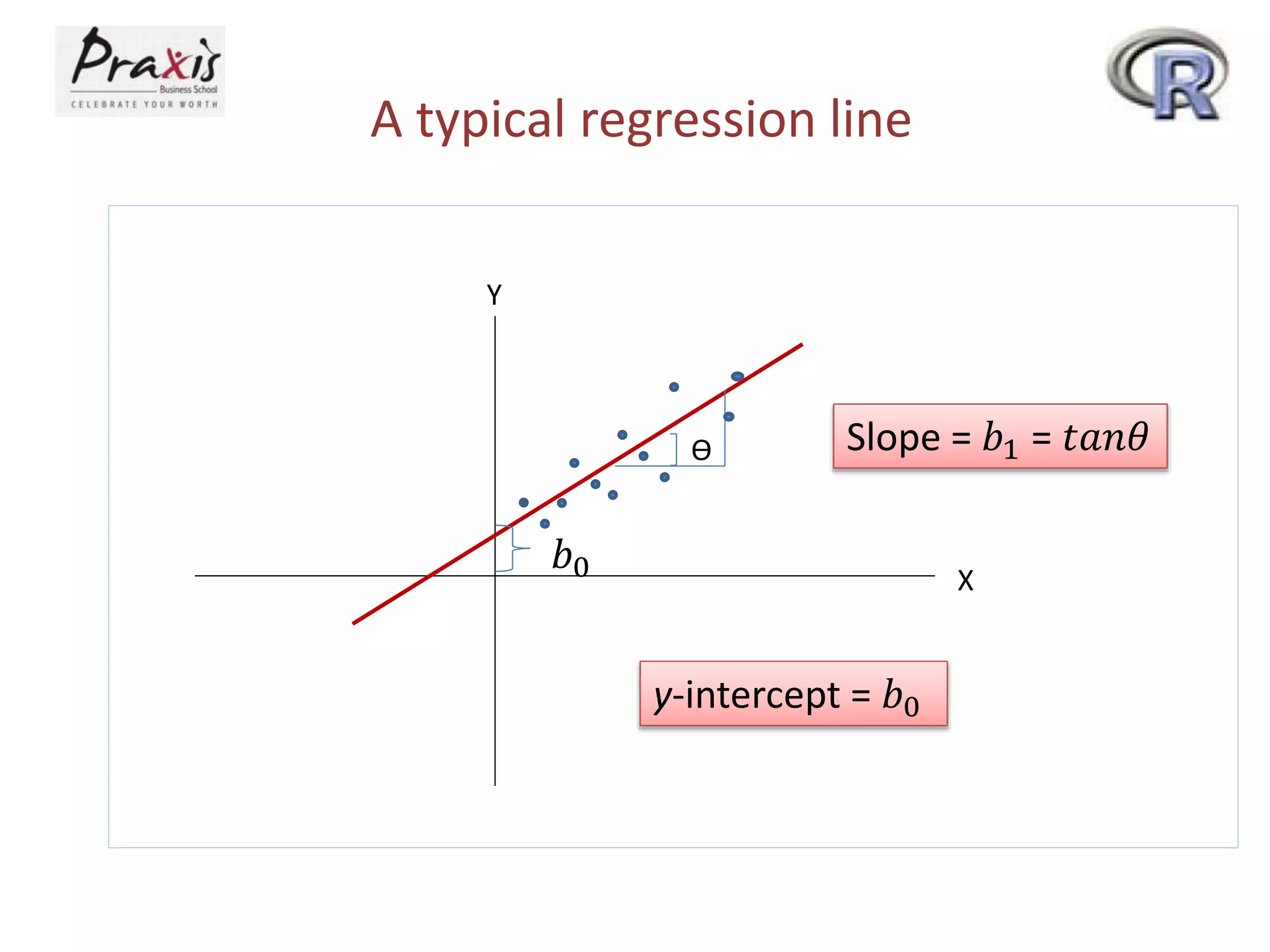
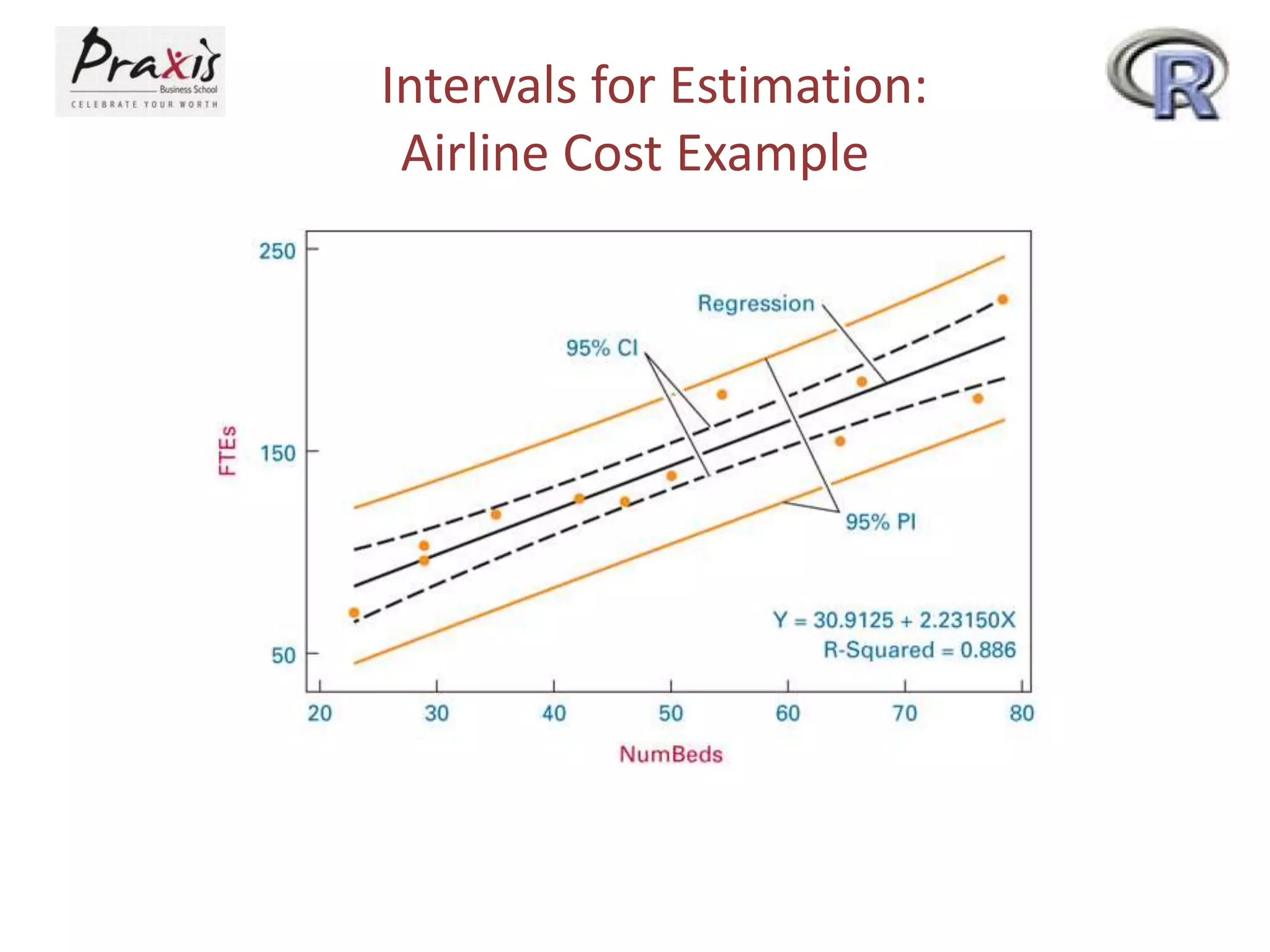
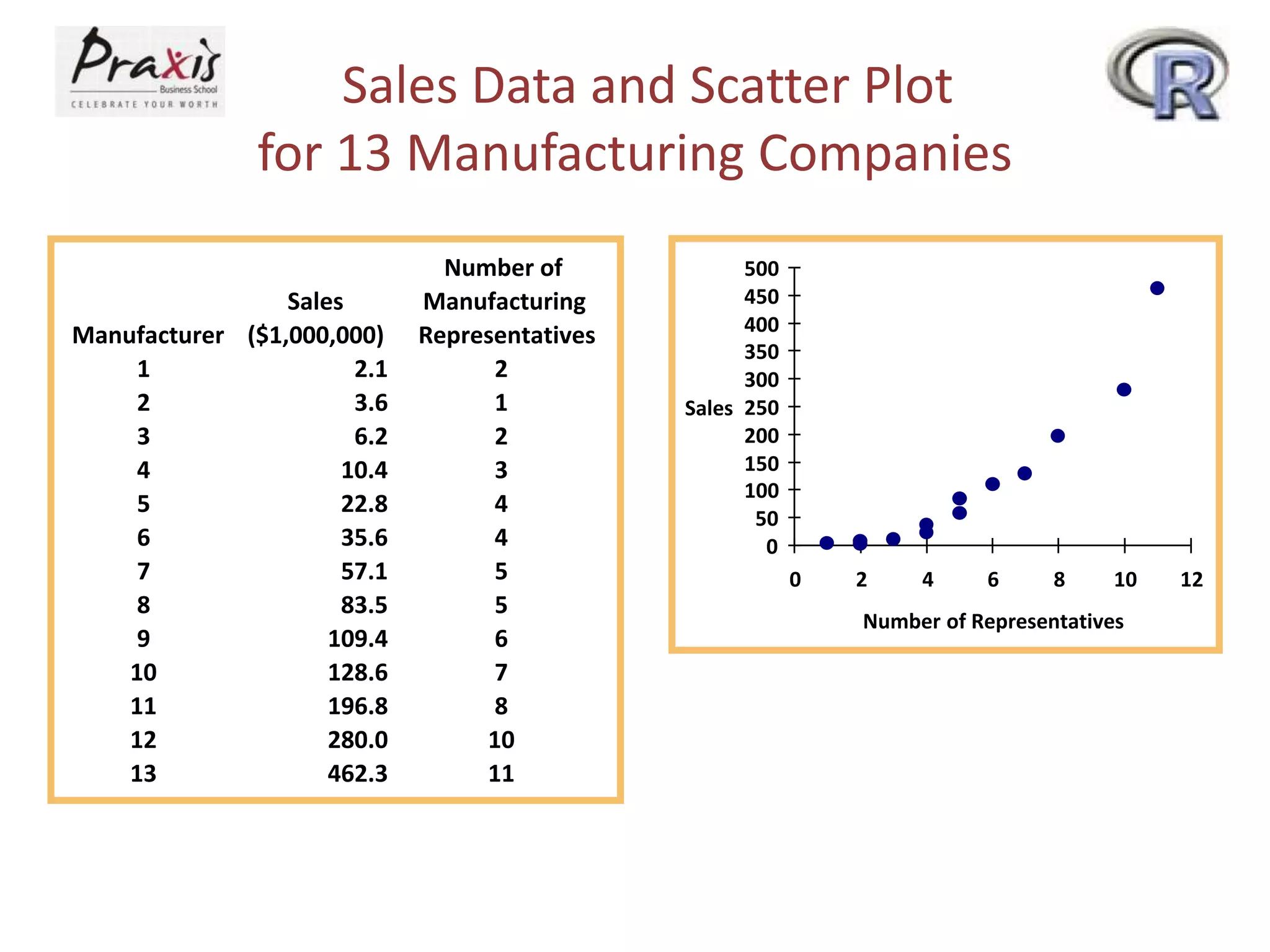
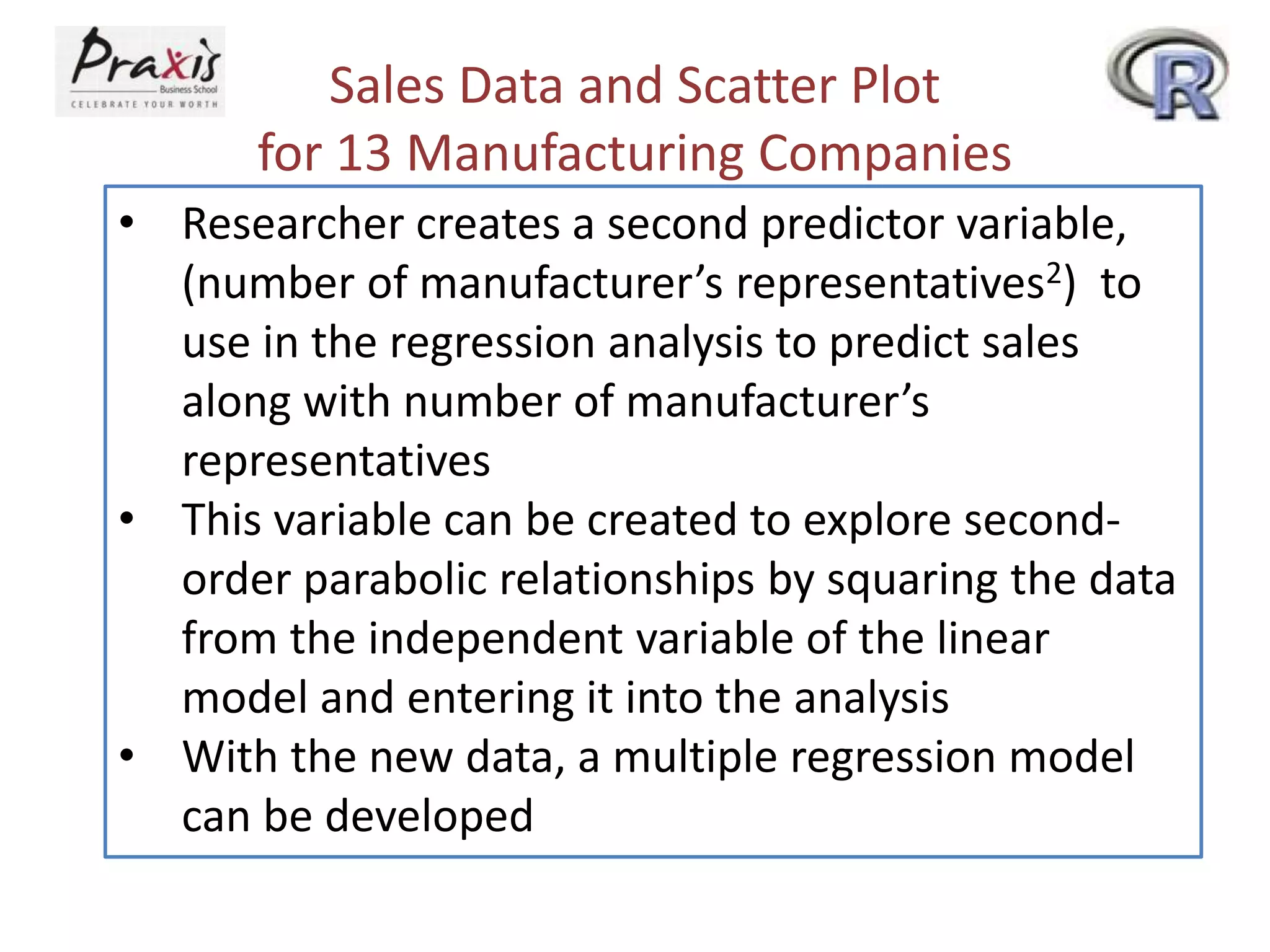
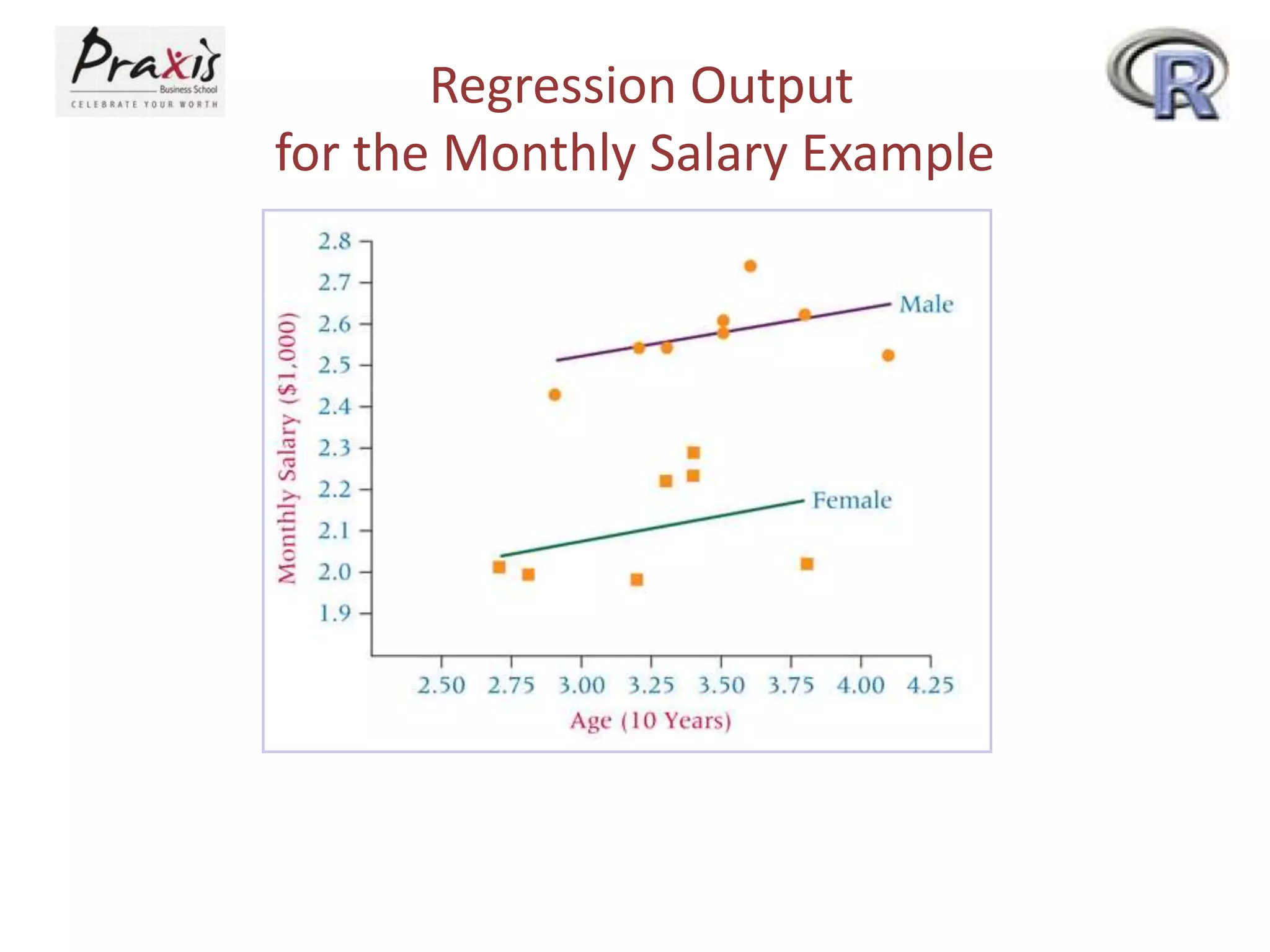
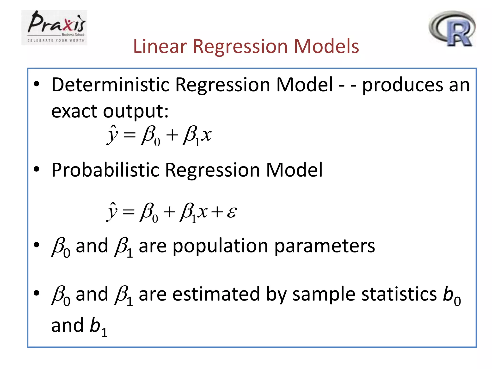
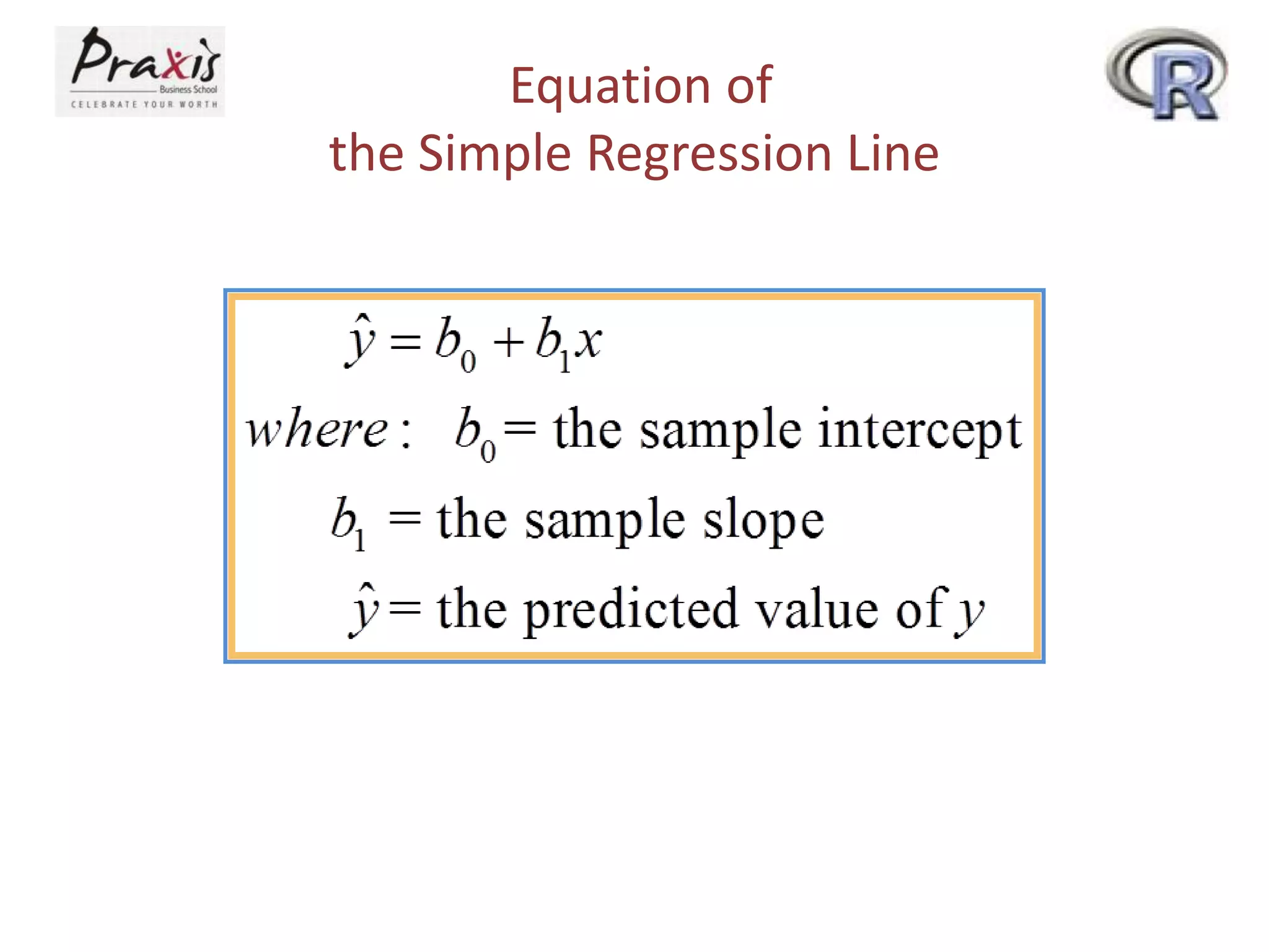
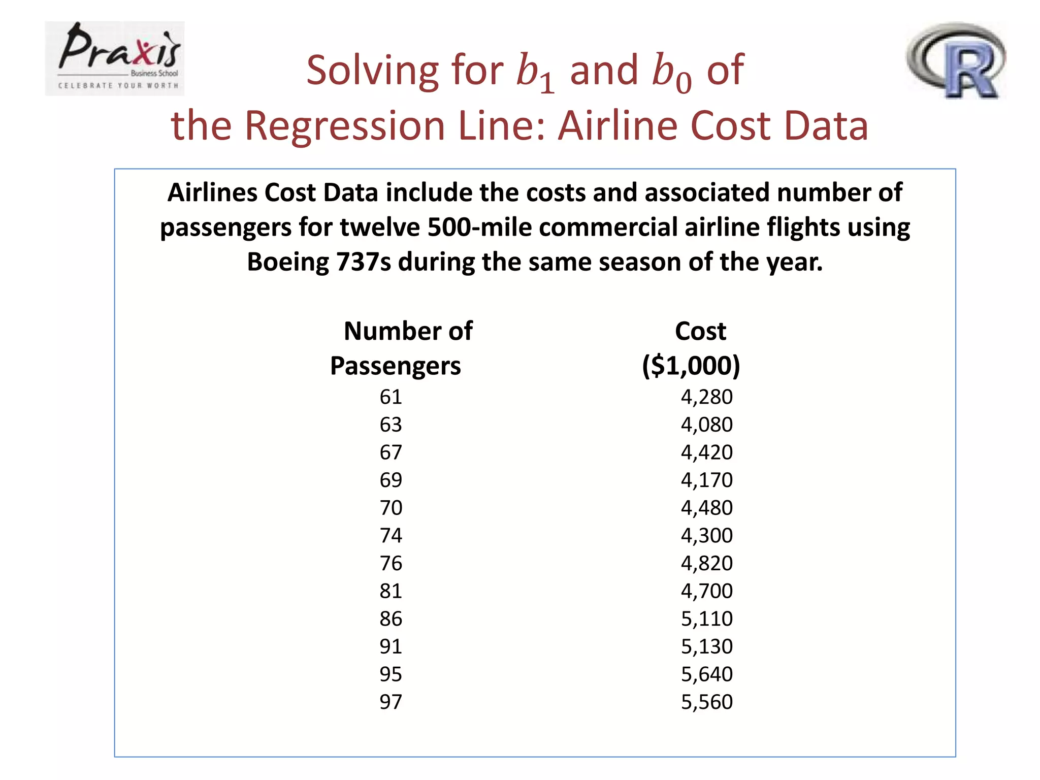
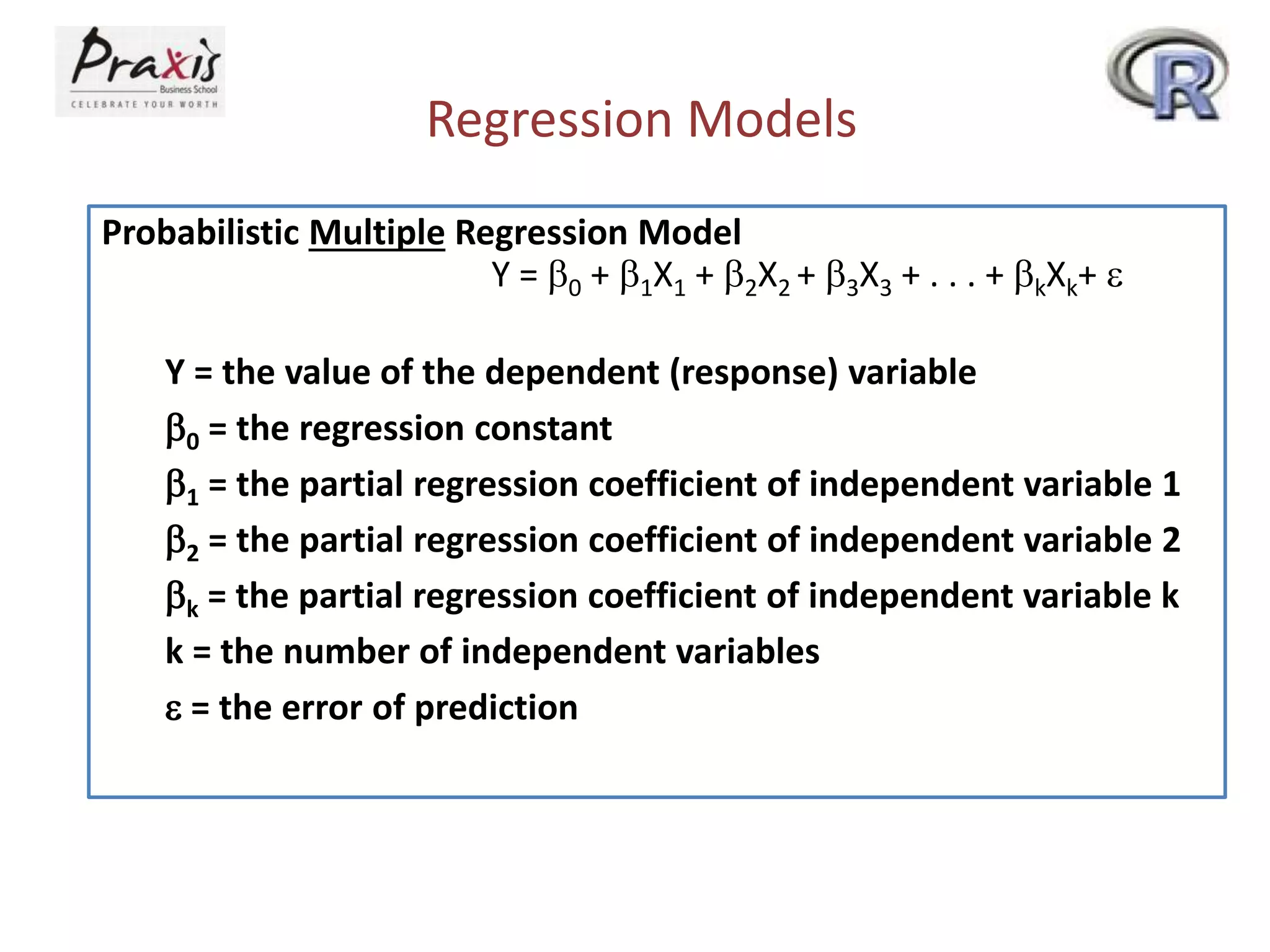
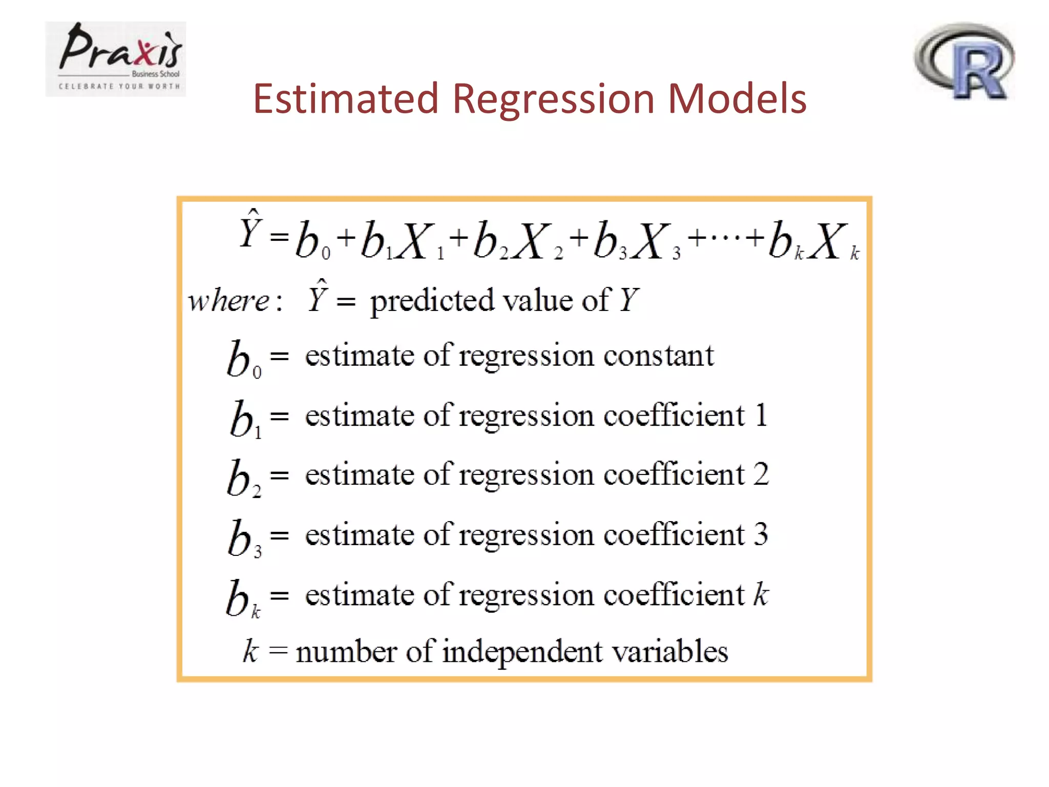
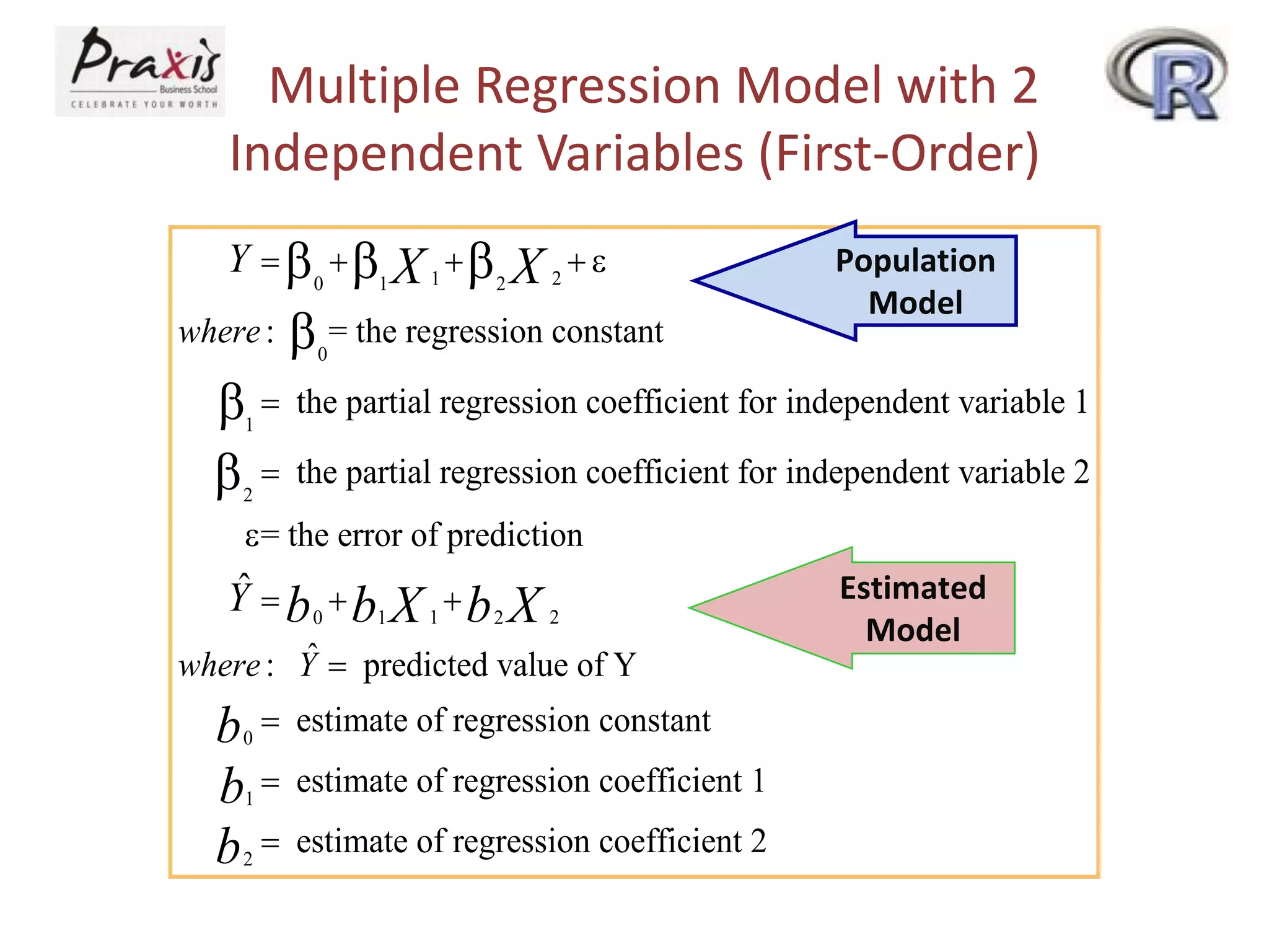
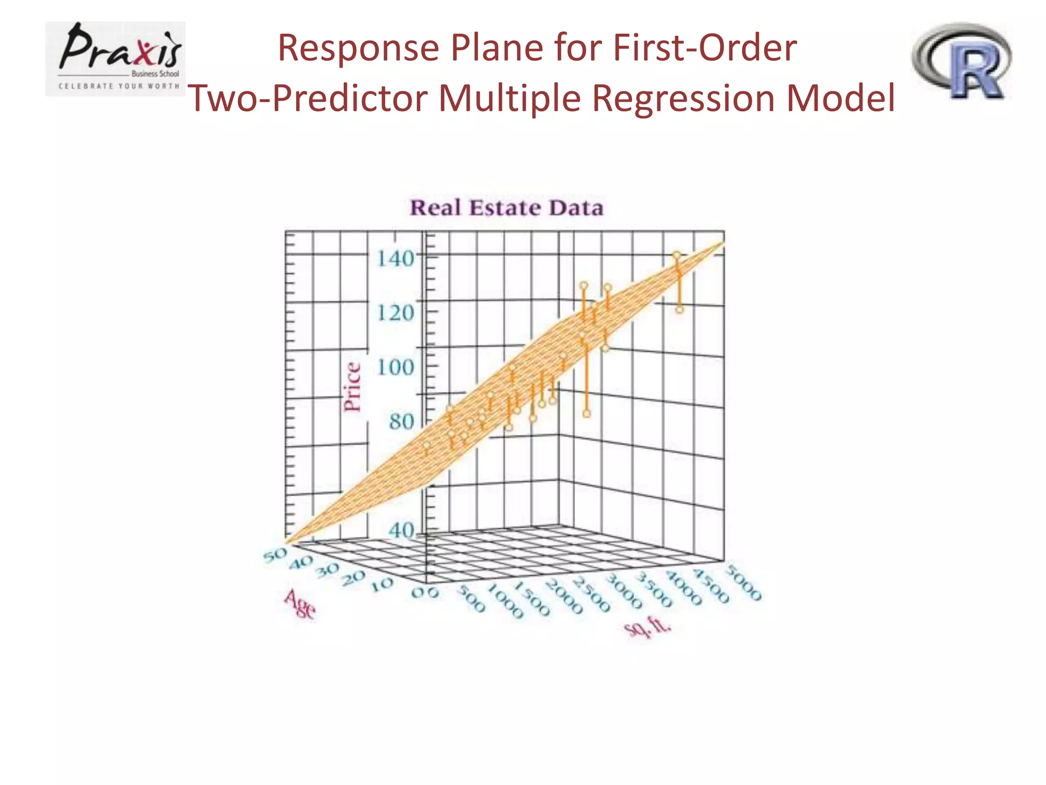
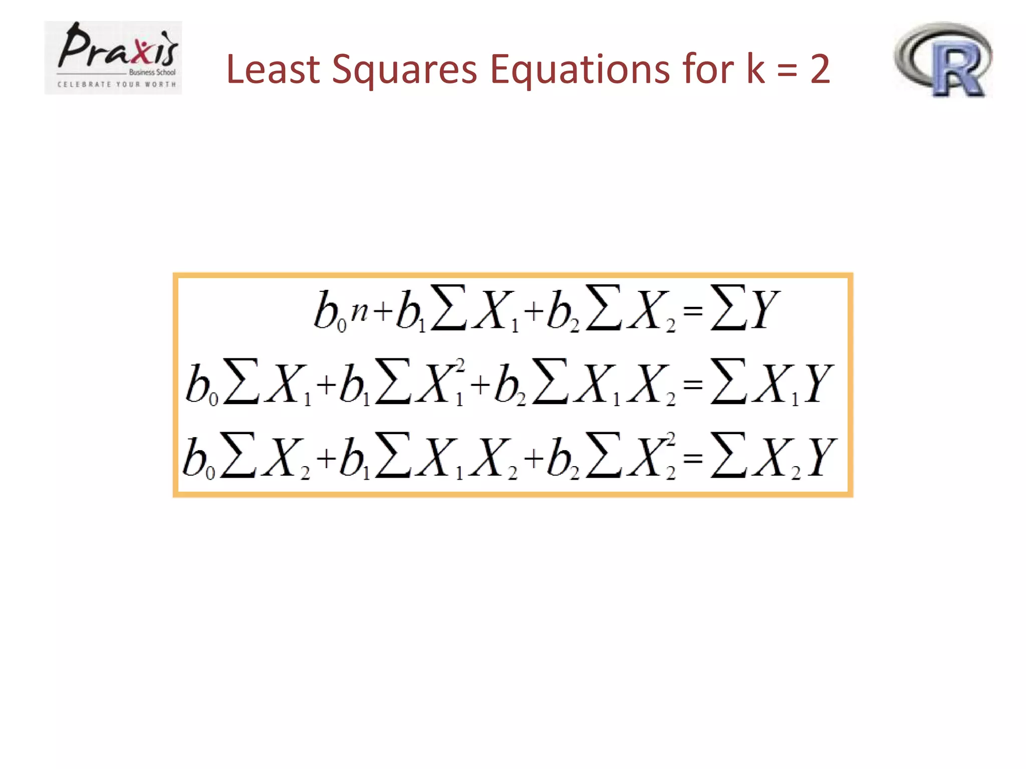
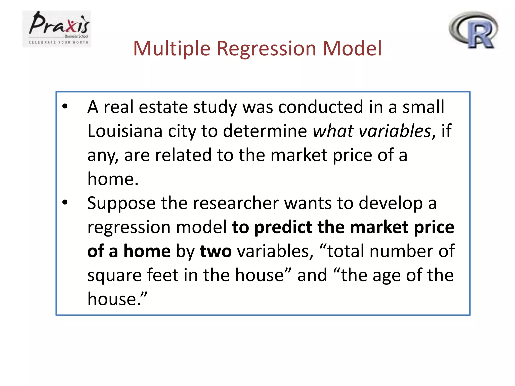
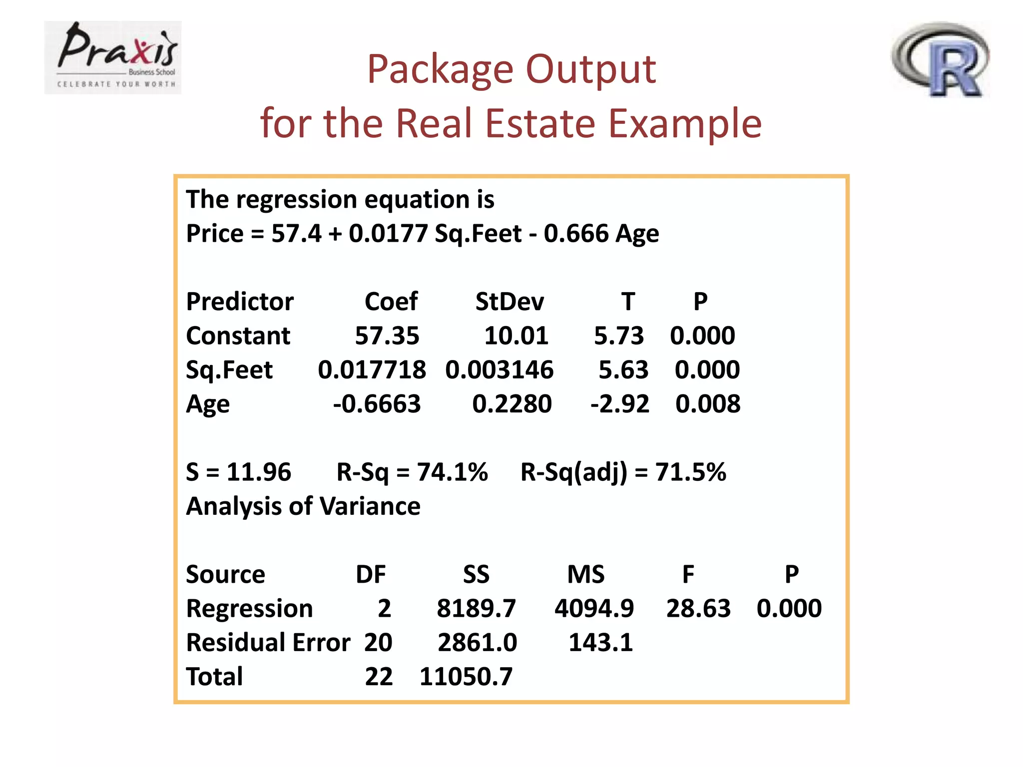
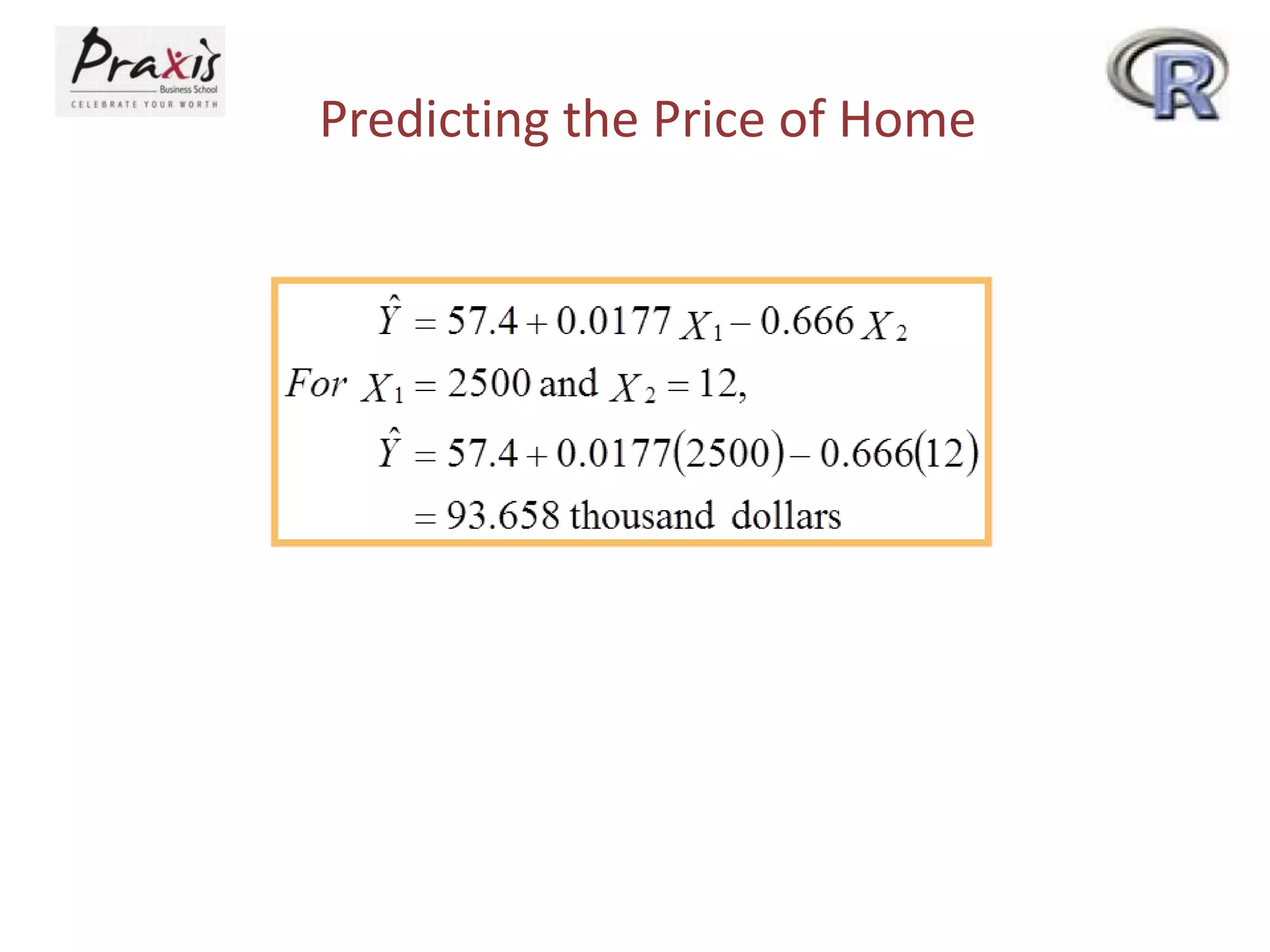
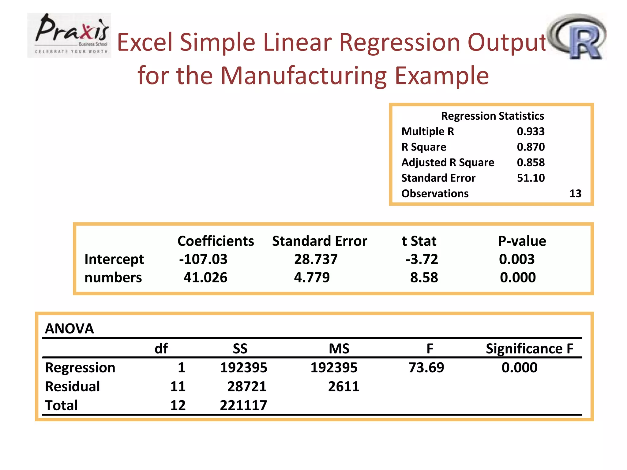
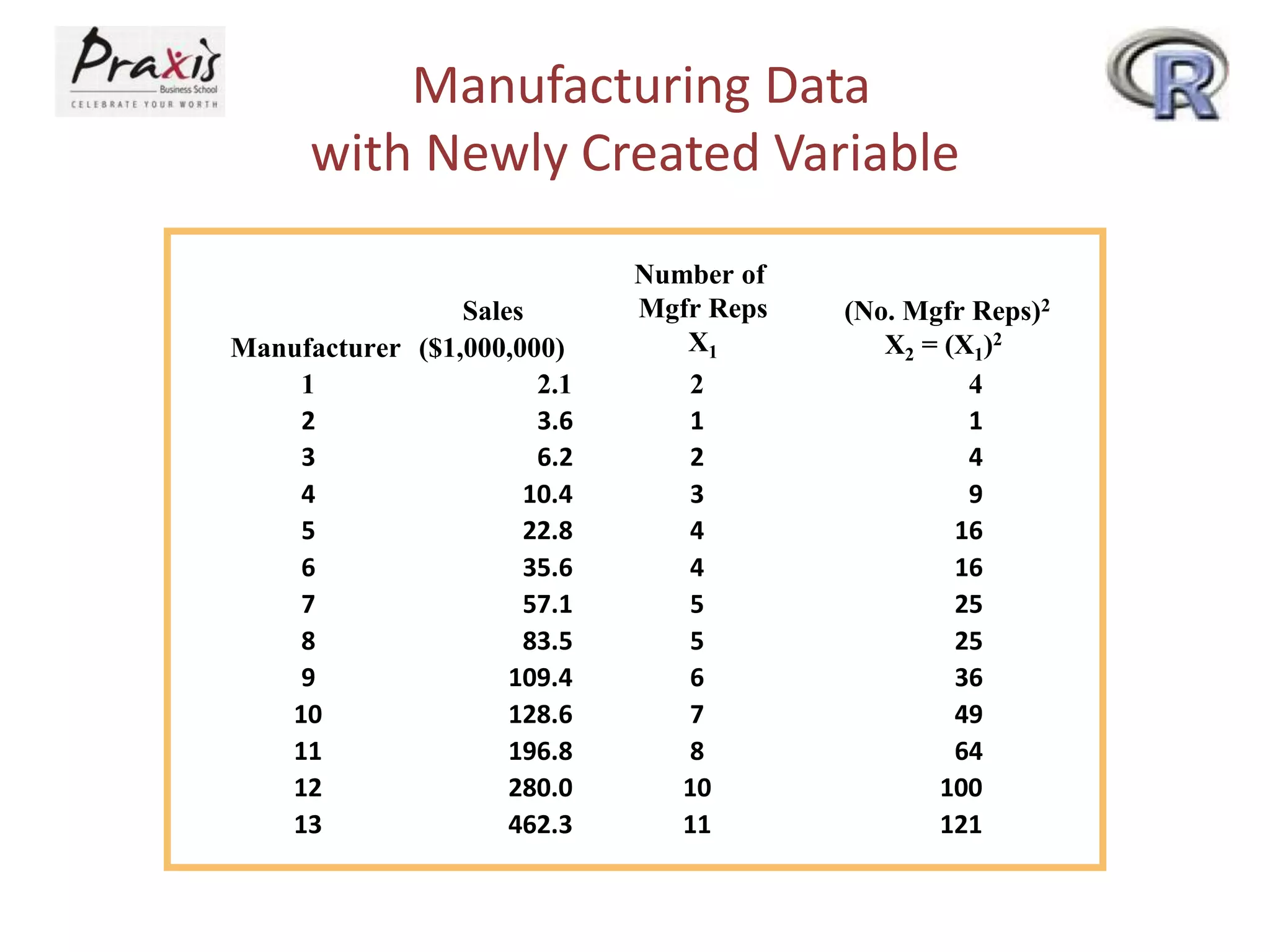
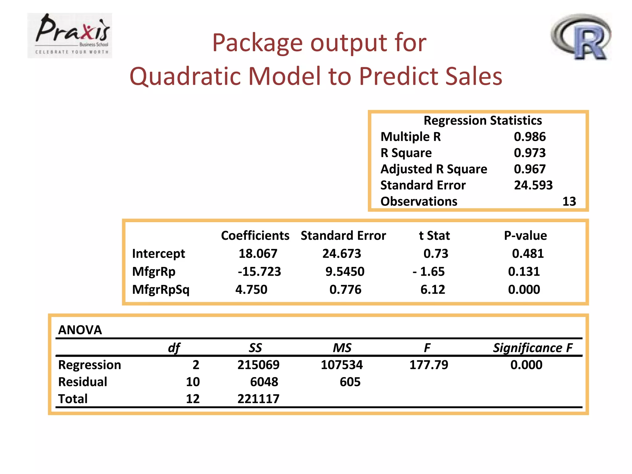
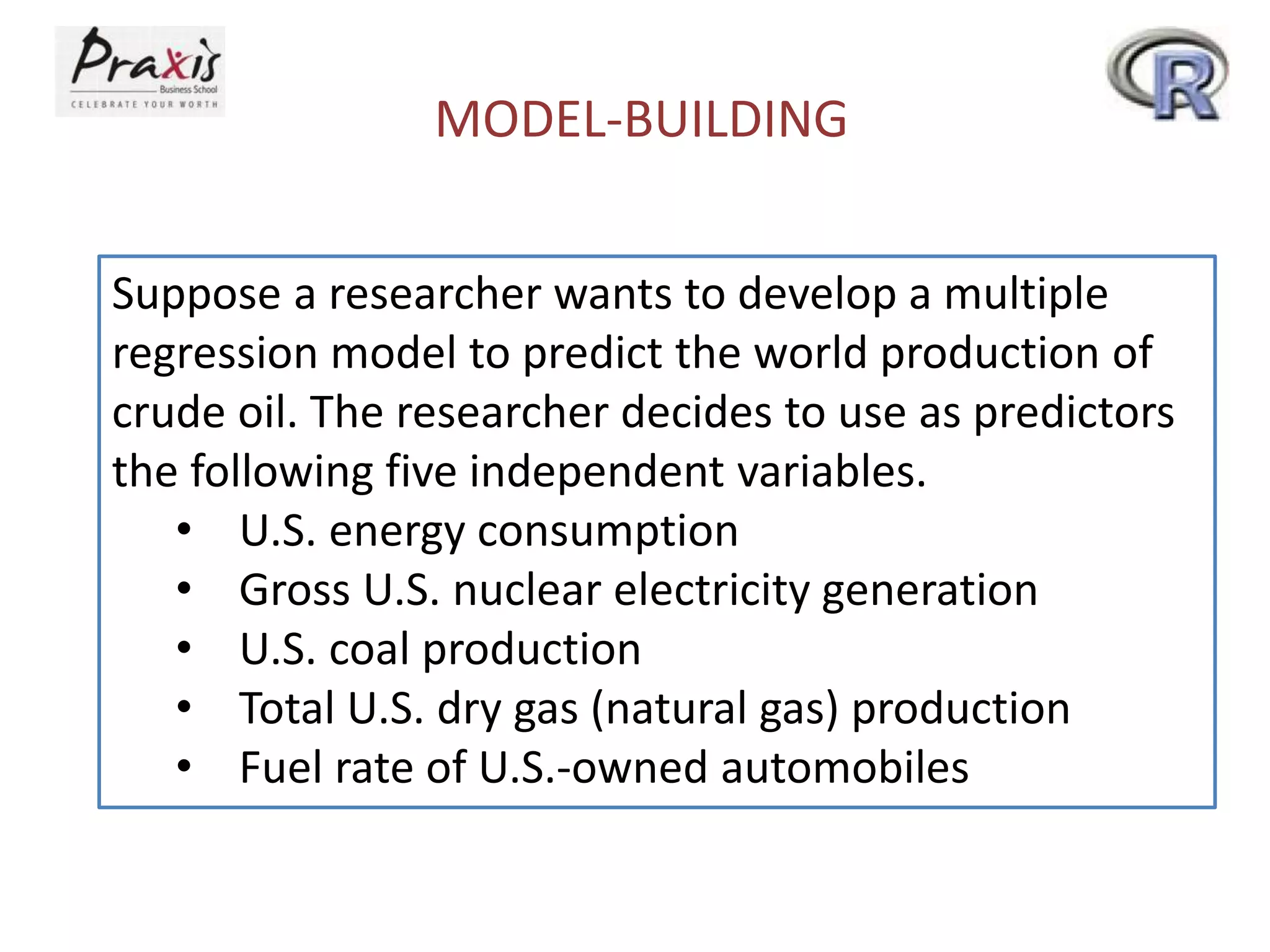
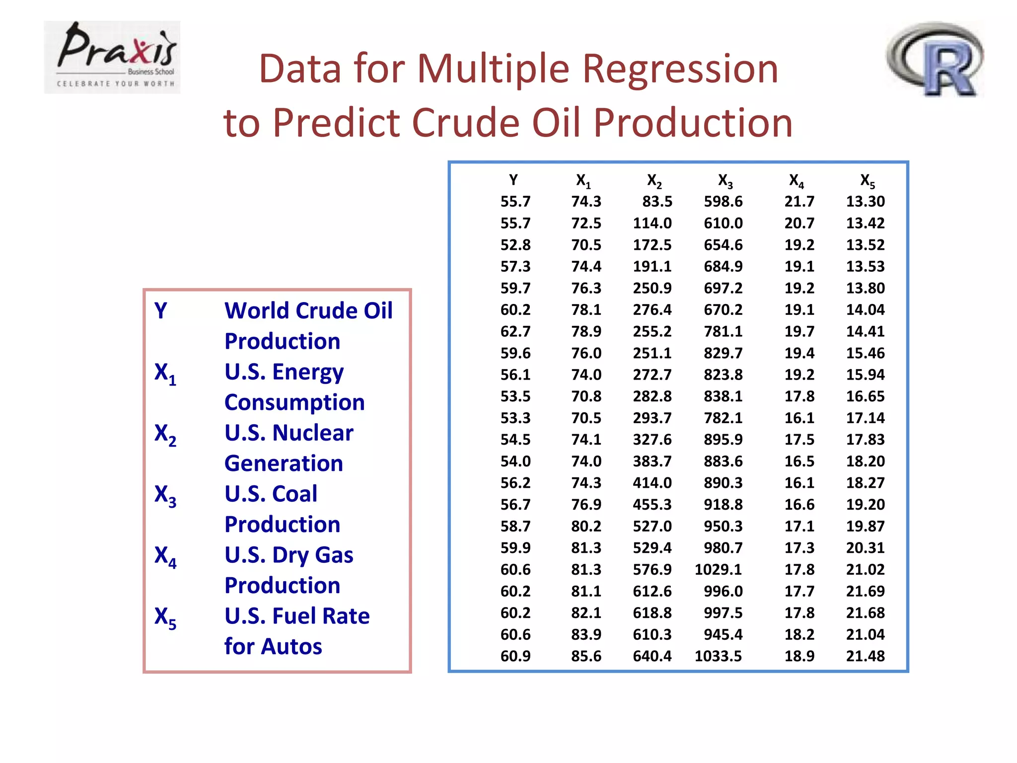
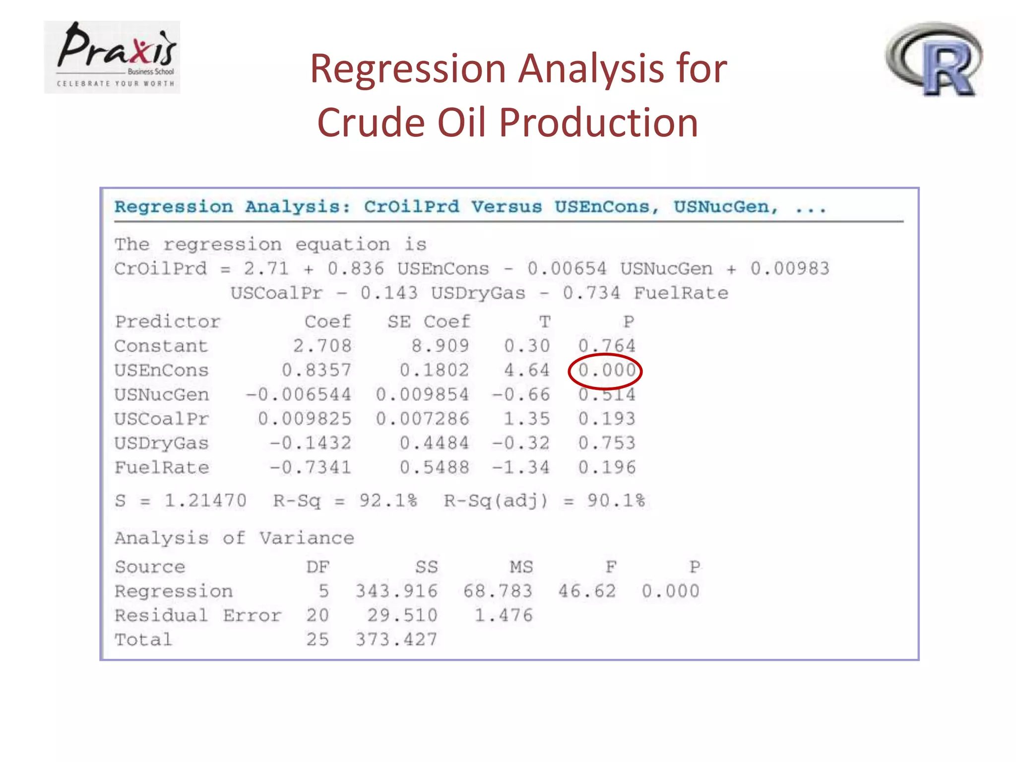
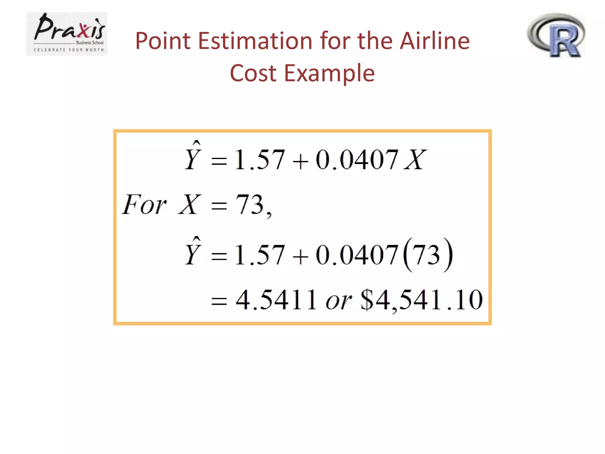
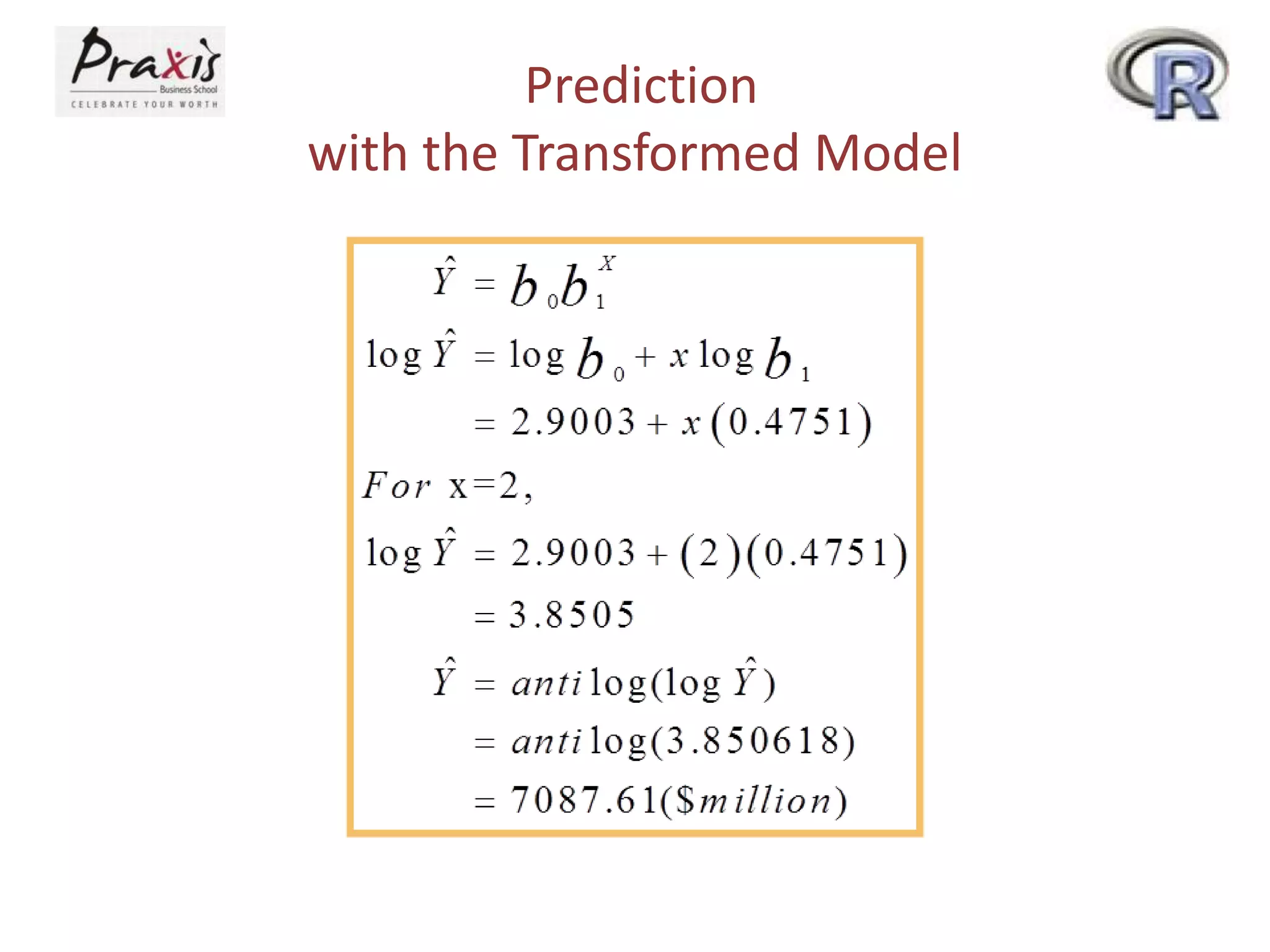
This document provides an overview of simple and multiple linear regression analysis. 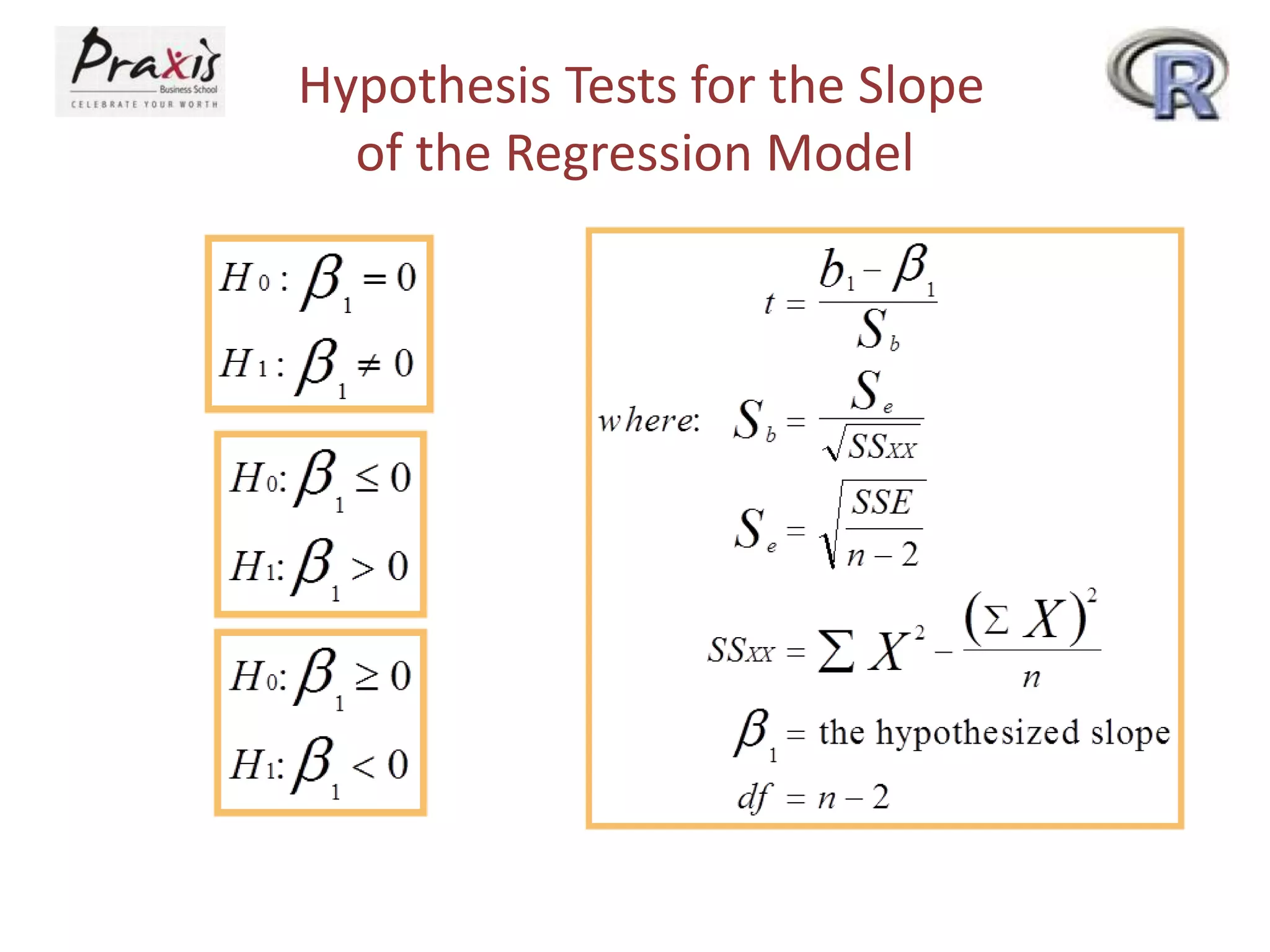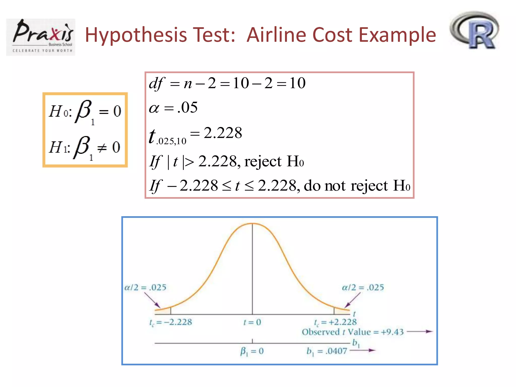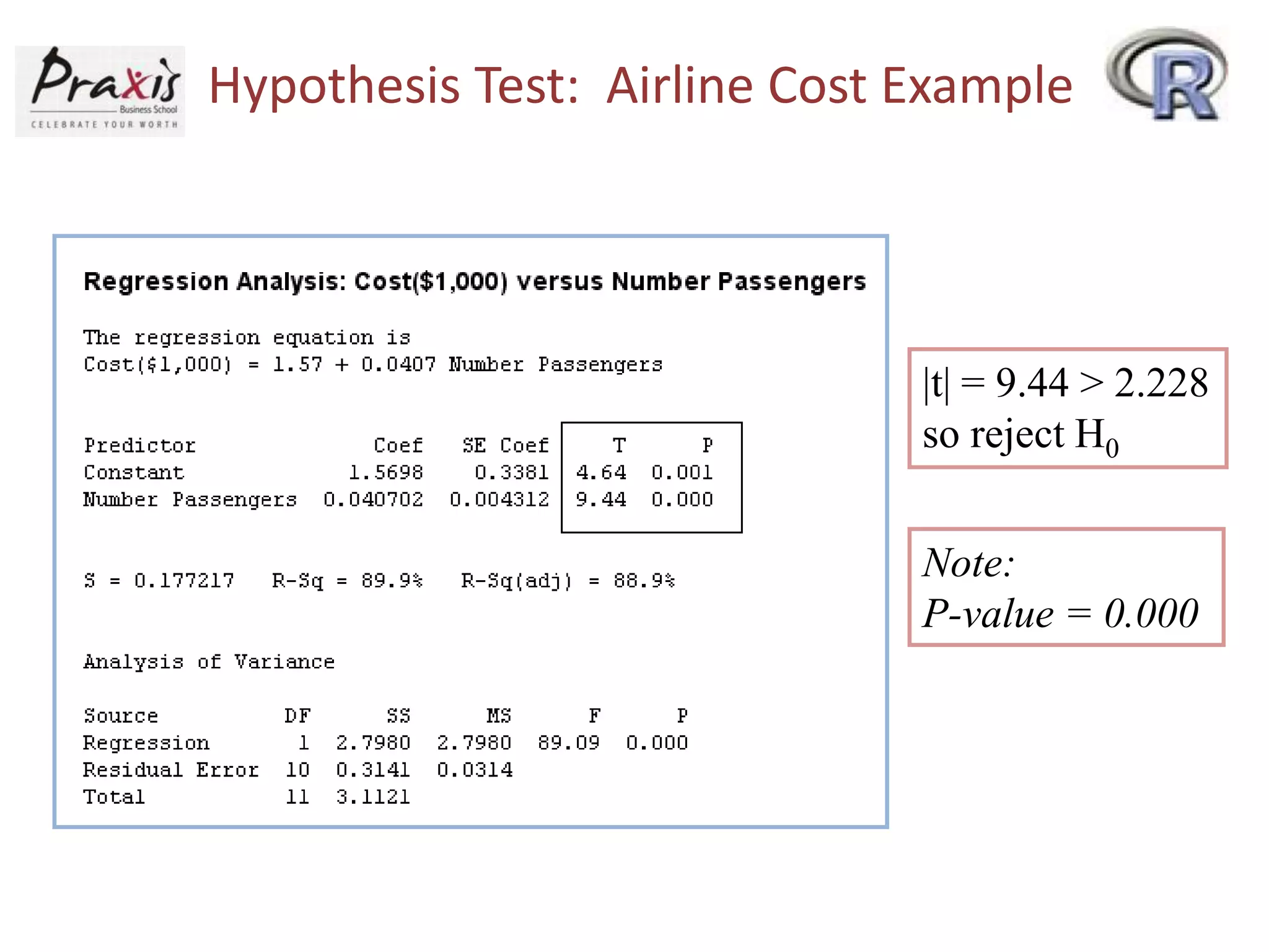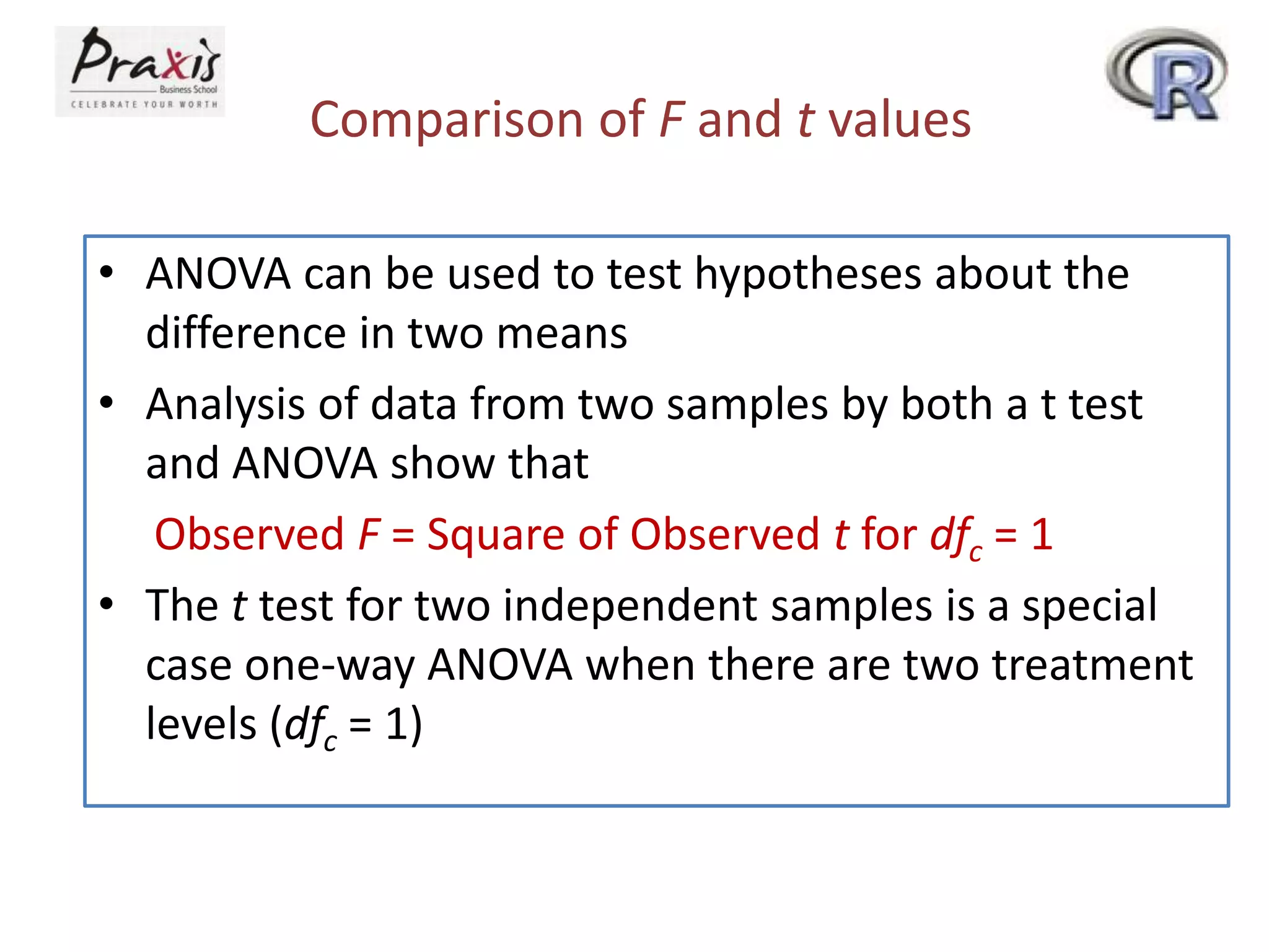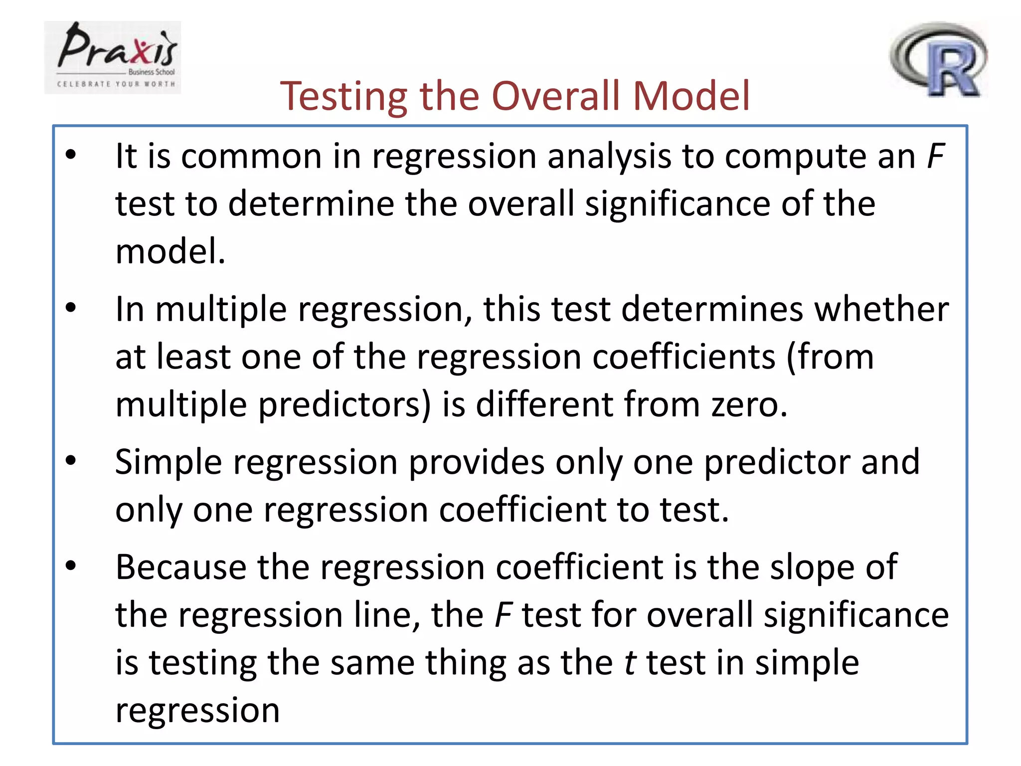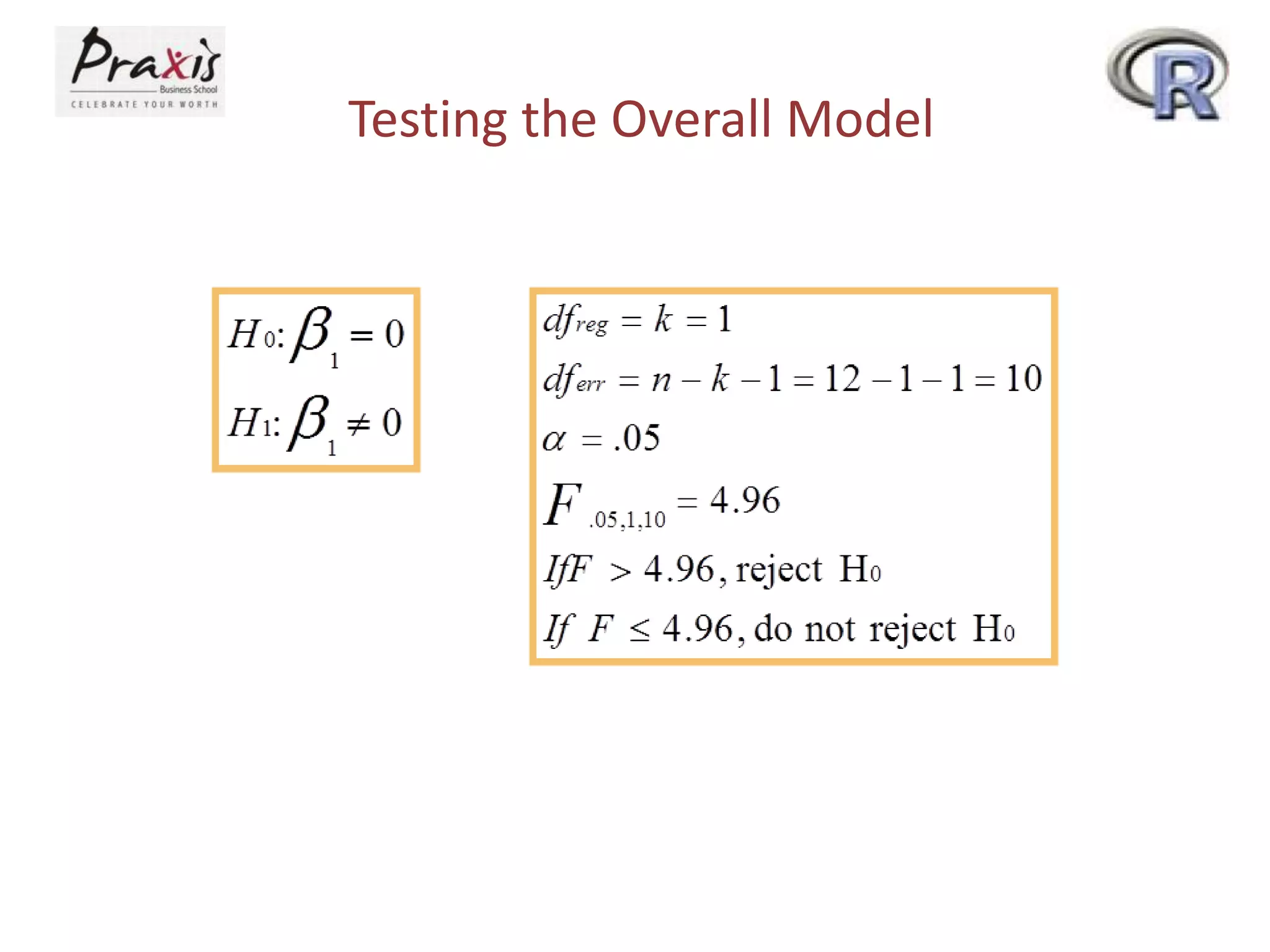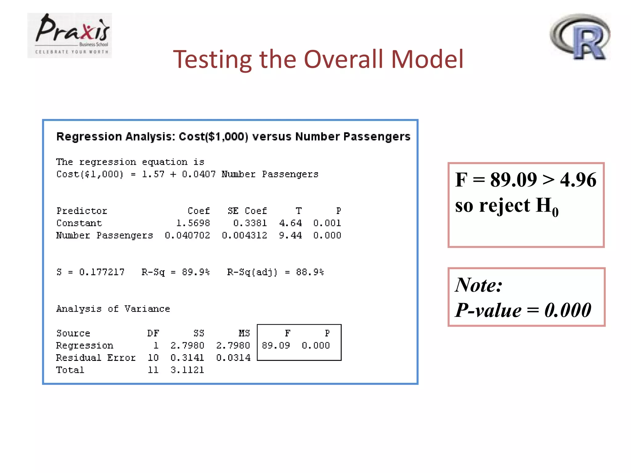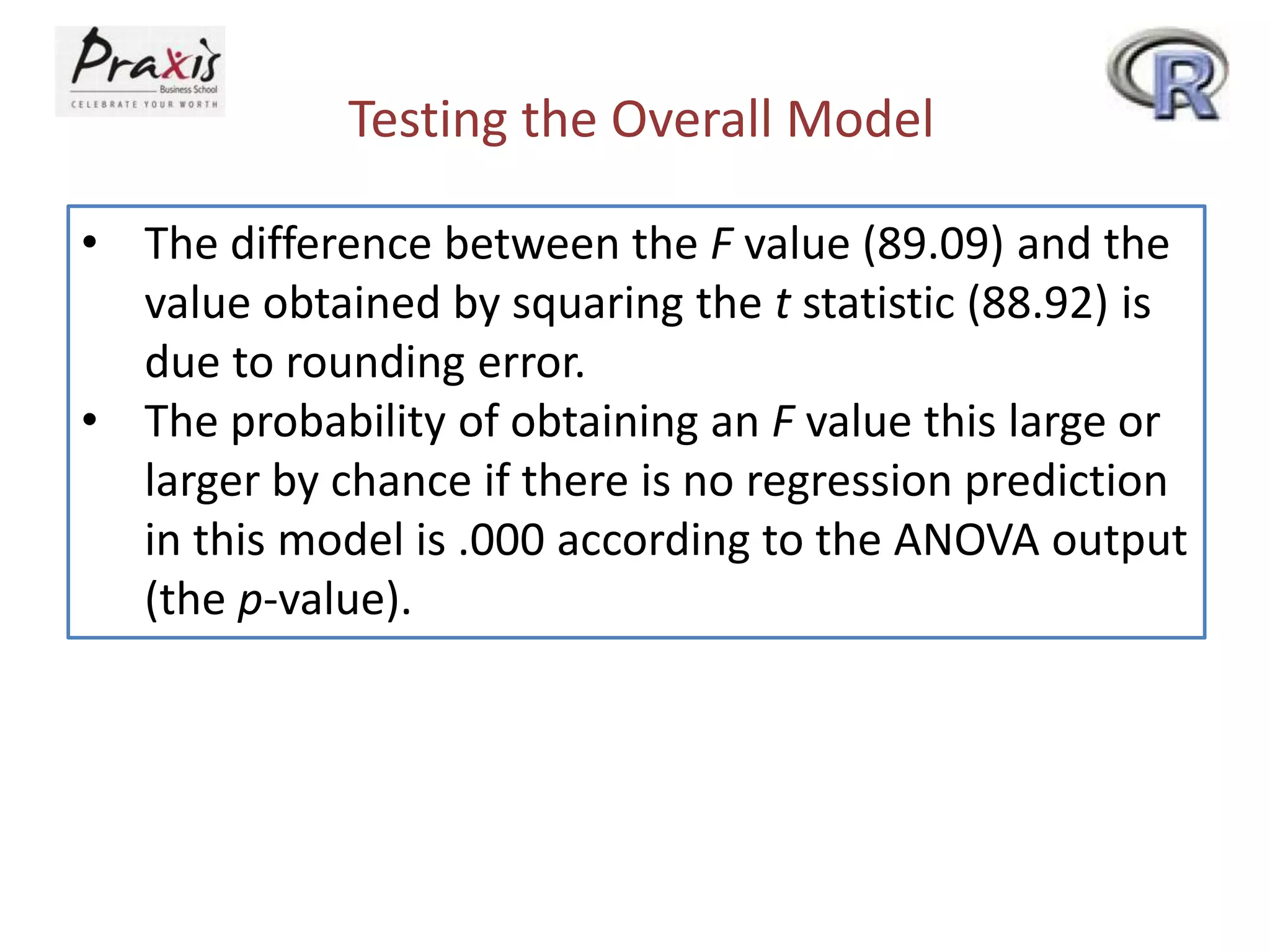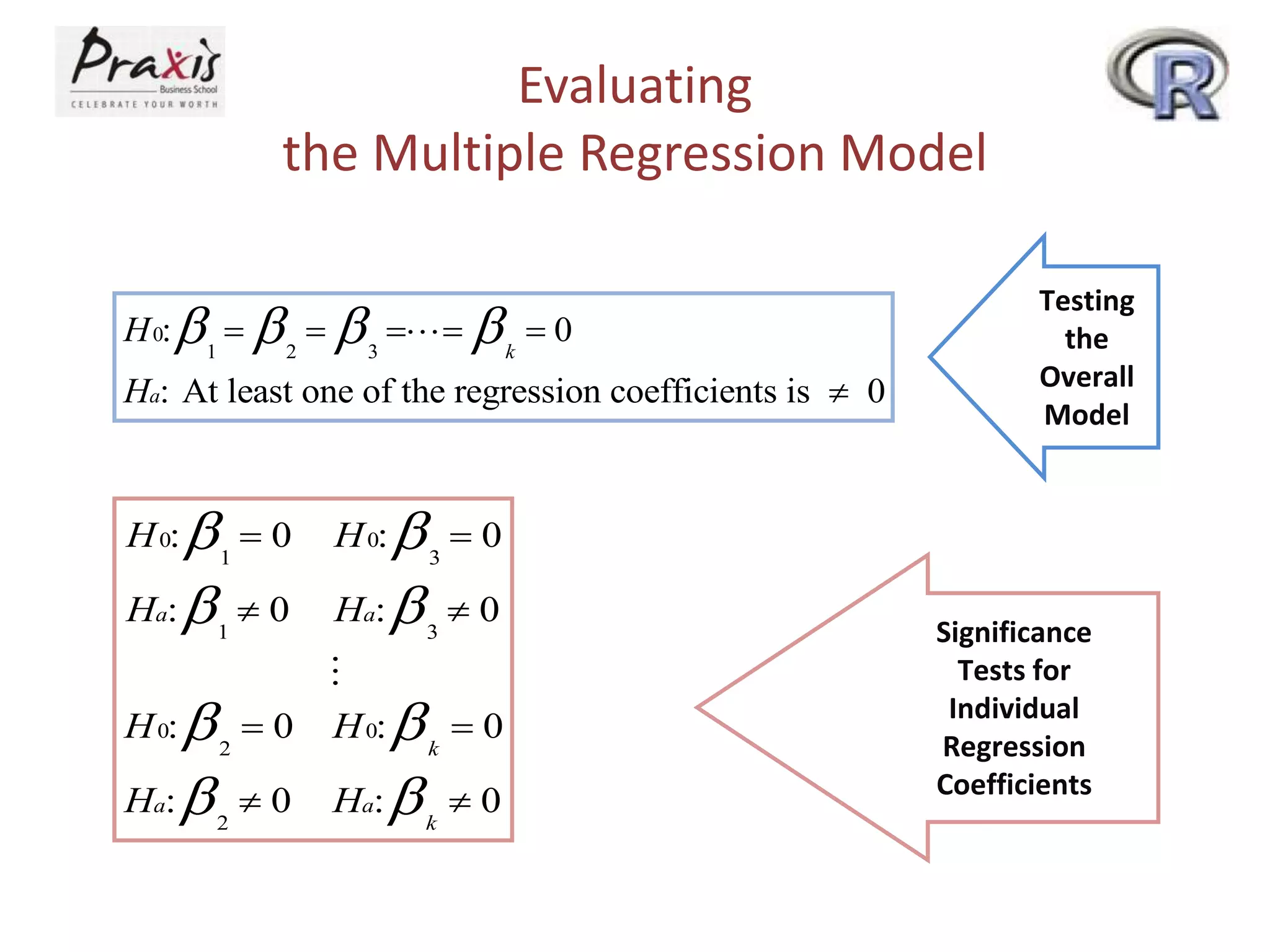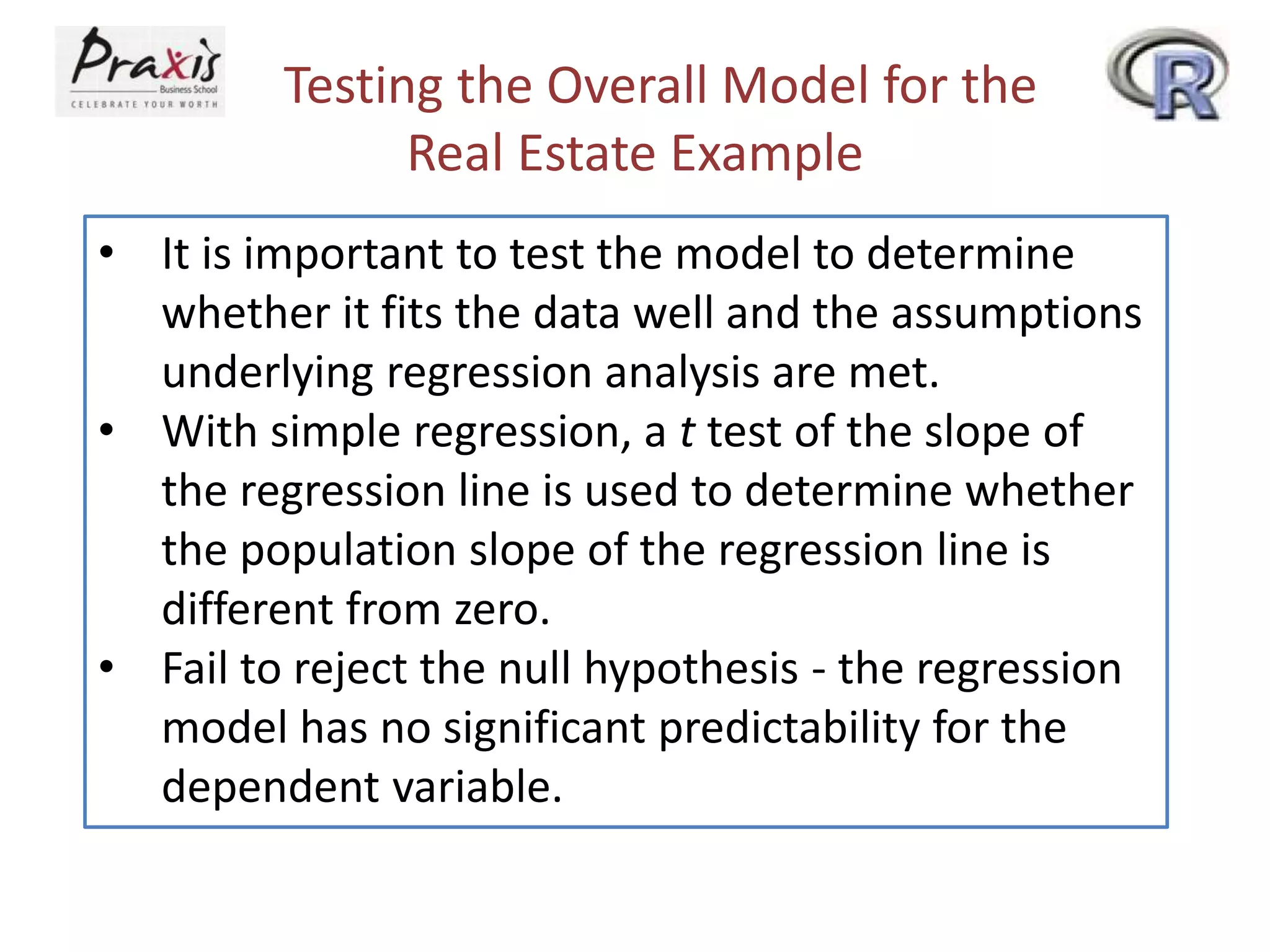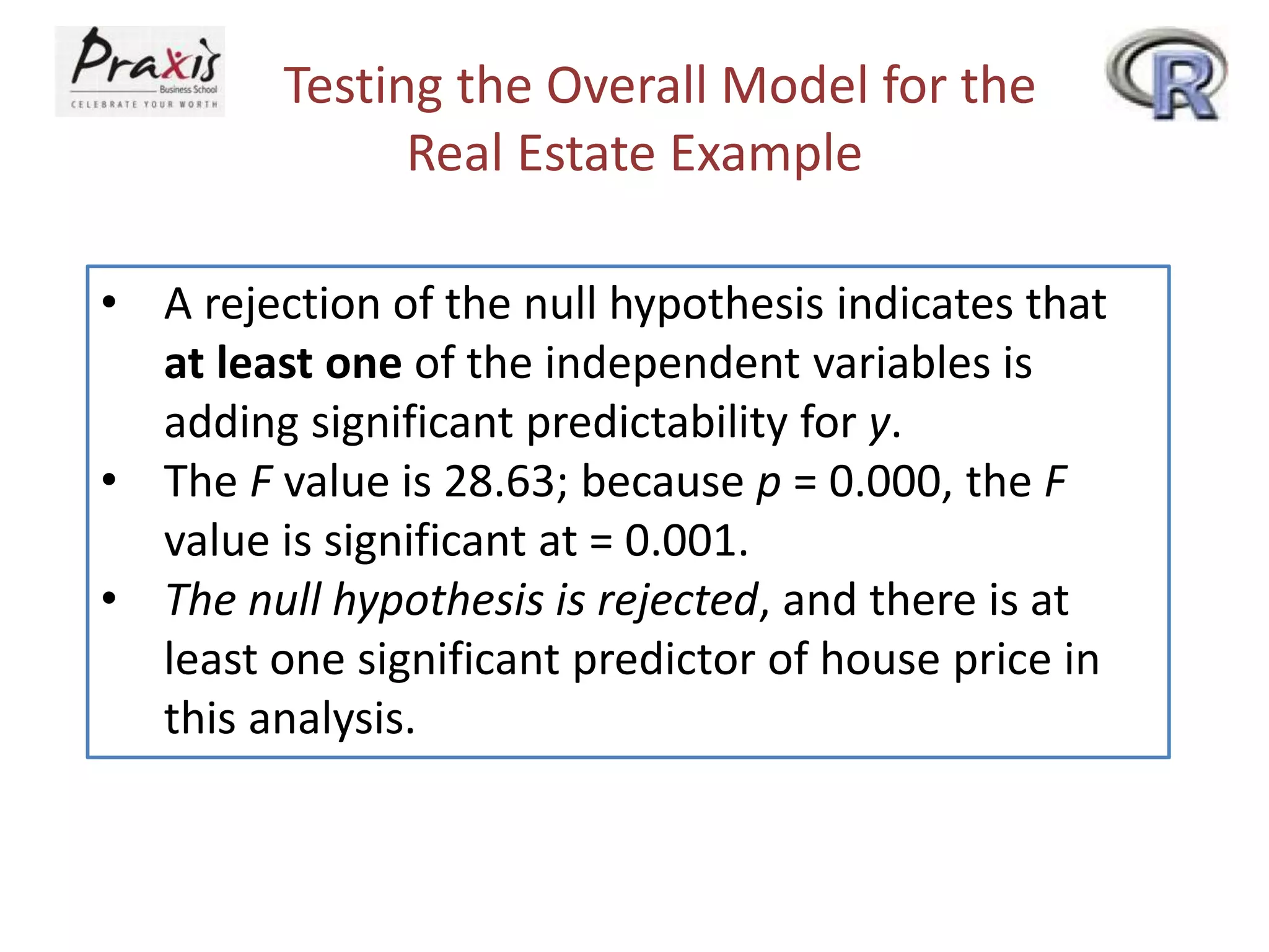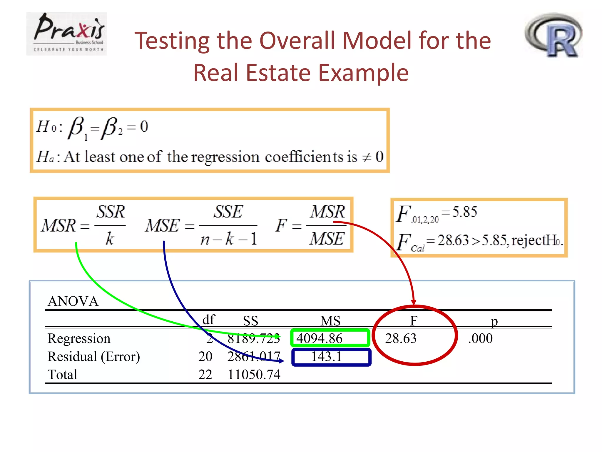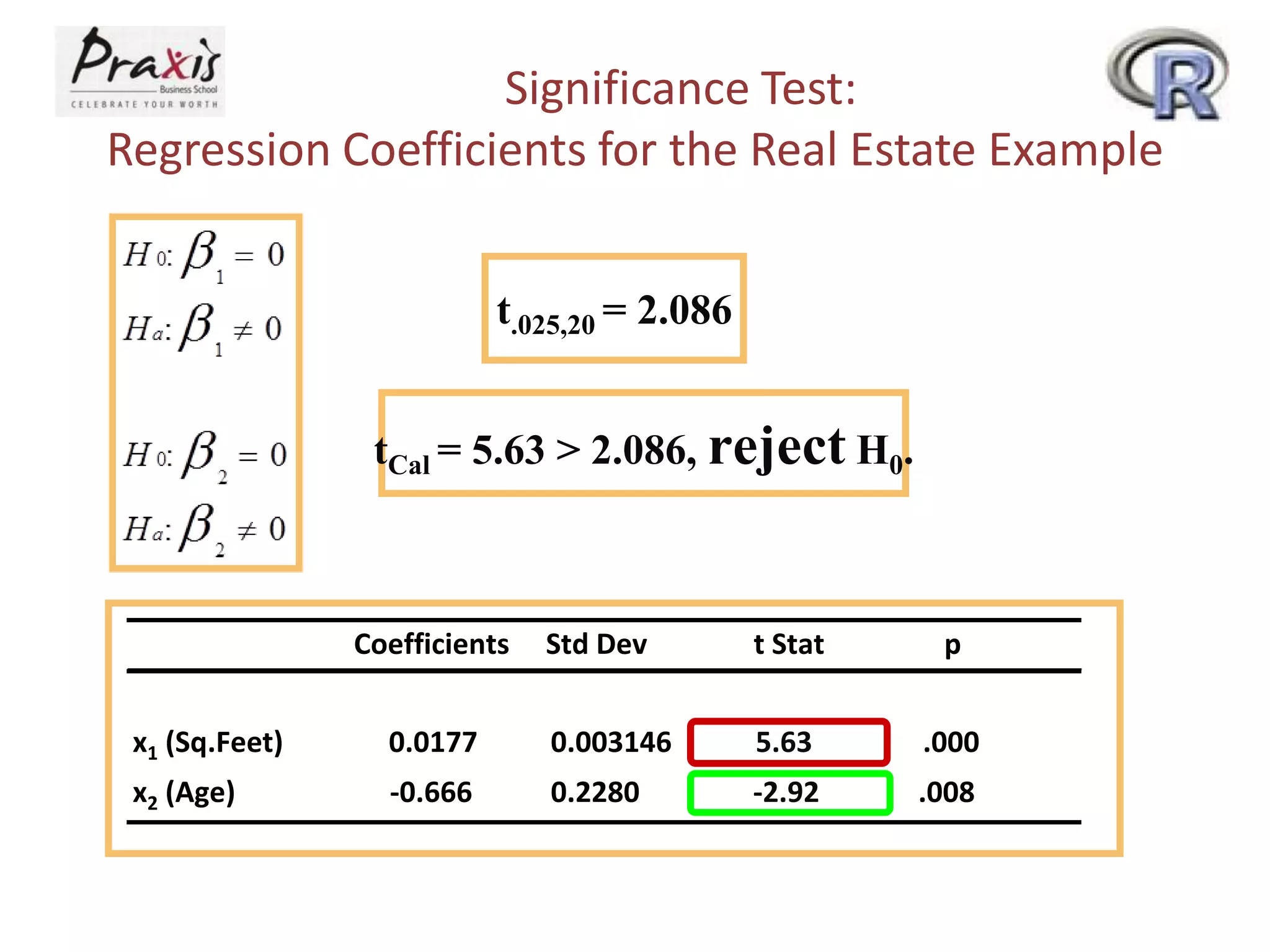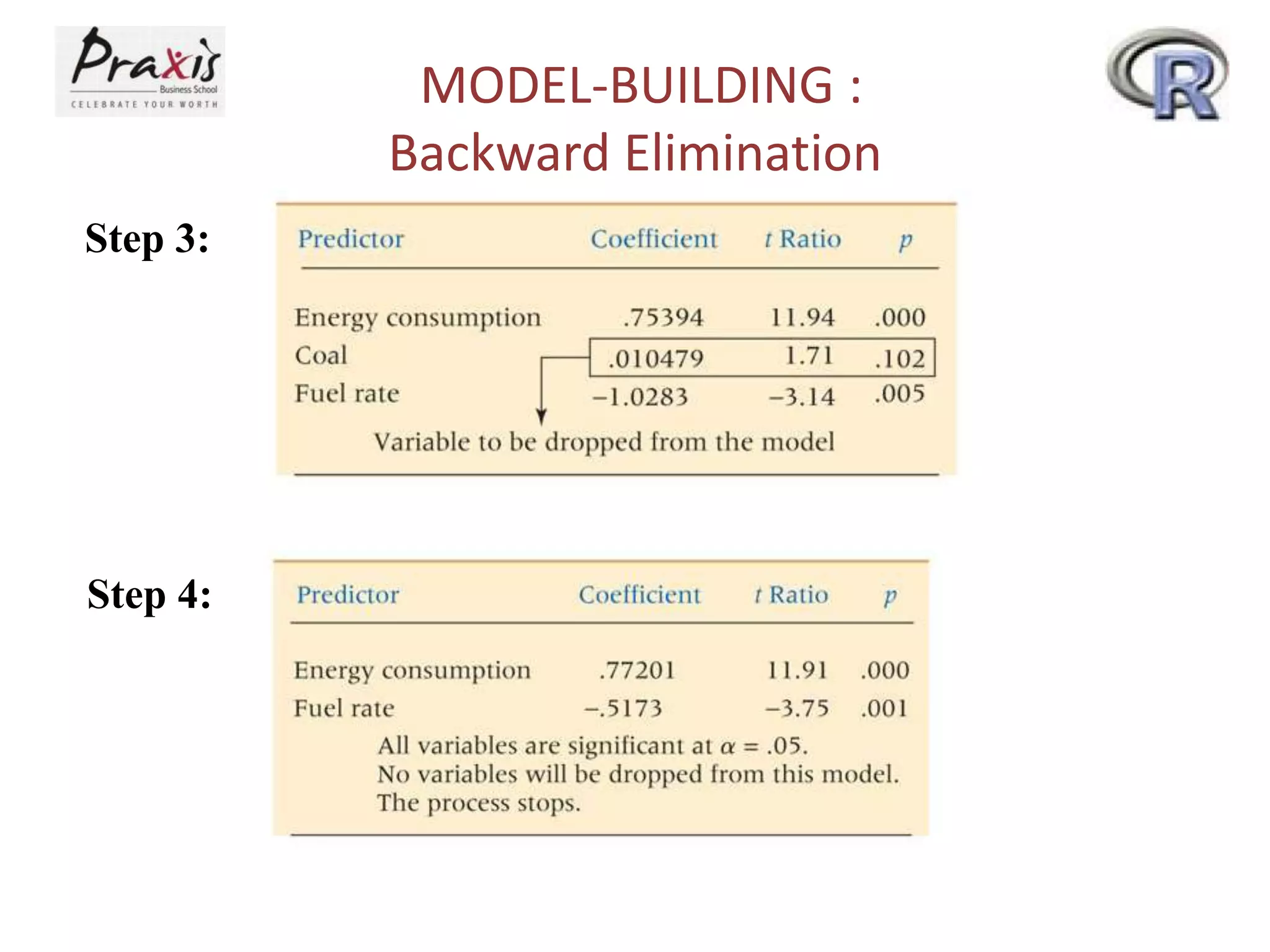It discusses key concepts such as: - Dependent and independent variables in bivariate linear regression - Using scatter plots to explore relationships - Estimating regression coefficients and equations for simple and multiple regression models - Using regression models to predict outcomes based on independent variable values - Conducting statistical tests on overall regression models and individual coefficients

1. Simple Regression Analysis
• Bivariate (two variables) linear regression -- the
most elementary regression model
– dependent variable, the variable to be predicted,
usually called Y
– independent variable, the predictor or explanatory
variable, usually called X
– Usually the first step in this analysis is to construct a
scatter plot of the data
• Nonlinear relationships and regression models
with more than one independent variable can be
explored by using multiple regression models

2. Linear Regression Models
• Deterministic Regression Model - - produces an
exact output:
• Probabilistic Regression Model
• 0 and 1 are population parameters
• 0 and 1 are estimated by sample statistics b0
and b1
0 1
ˆy x  
0 1
ˆy x    

3. Equation of
the Simple Regression Line

4. A typical regression line
X
Y
𝑏0
ϴ Slope = 𝑏1 = 𝑡𝑎𝑛𝜃
y-intercept = 𝑏0

5. Hypothesis Tests for the Slope
of the Regression Model
• A hypothesis test can be conducted on the sample
slope of the regression model to determine
whether the population slope is significantly
different from zero.
• Using the non-regression model (the 𝑦 model) as a
worst case, the researcher can analyze the
regression line to determine whether it adds a
more significant amount of predictability of y than
does the model.

6. Hypothesis Tests for the Slope
of the Regression Model
• As the slope of the regression line diverges from
zero, the regression model is adding predictability
that the line is not generating.
• Testing the slope of the regression line to determine
whether the slope is different from zero is important.
• If the slope is not different from zero, the regression
line is doing nothing more than the average line of y
predicting y 𝑦 model

7. Hypothesis Tests for the Slope
of the Regression Model

8. Solving for 𝑏1 and 𝑏0 of
the Regression Line: Airline Cost Data
Airlines Cost Data include the costs and associated number of
passengers for twelve 500-mile commercial airline flights using
Boeing 737s during the same season of the year.
Number of Cost
Passengers ($1,000)
61 4,280
63 4,080
67 4,420
69 4,170
70 4,480
74 4,300
76 4,820
81 4,700
86 5,110
91 5,130
95 5,640
97 5,560

9. Hypothesis Test: Airline Cost Example
0
0
10,025.
Hrejectnotdo,228.2228.2
Hreject,228.2||
228.2
05.
102102





tIf
tIf
ndf
t


10. Hypothesis Test: Airline Cost Example
|t| = 9.44 > 2.228
so reject H0
Note:
P-value = 0.000

11. Hypothesis Test:
Airline Cost Example
• The t value calculated from the sample slope falls in
the rejection region and the p-value is .00000014.
• The null hypothesis that the population slope is zero
is rejected.
• This linear regression model is adding significantly
more predictive information to the model (no
regression).

12. Comparison of F and t values
• ANOVA can be used to test hypotheses about the
difference in two means
• Analysis of data from two samples by both a t test
and ANOVA show that
Observed F = Square of Observed t for dfc = 1
• The t test for two independent samples is a special
case one-way ANOVA when there are two treatment
levels (dfc = 1)

13. Testing the Overall Model
• It is common in regression analysis to compute an F
test to determine the overall significance of the
model.
• In multiple regression, this test determines whether
at least one of the regression coefficients (from
multiple predictors) is different from zero.
• Simple regression provides only one predictor and
only one regression coefficient to test.
• Because the regression coefficient is the slope of
the regression line, the F test for overall significance
is testing the same thing as the t test in simple
regression

14. Testing the Overall Model

15. Testing the Overall Model
F = 89.09 > 4.96
so reject H0
Note:
P-value = 0.000

16. Testing the Overall Model
• The difference between the F value (89.09) and the
value obtained by squaring the t statistic (88.92) is
due to rounding error.
• The probability of obtaining an F value this large or
larger by chance if there is no regression prediction
in this model is .000 according to the ANOVA output
(the p-value).

17. Estimation
• One of the main uses of regression analysis is as a
prediction tool.
• If the regression function is a good model, the
researcher can use the regression equation to
determine values of the dependent variable from
various values of the independent variable.
• In simple regression analysis, a point estimate
prediction of y can be made by substituting the
associated value of x into the regression equation
and solving for y.

18. Point Estimation for the Airline
Cost Example

19. Confidence Interval of Estimate of
the Conditional Mean of y
• The regression line is determined by a sample set
of points. For different samples, the regression
equations will be different, yielding different Point
Estimates.
• Hence a Confidence Interval (CI) of estimation is
often useful because for any value of independent
variable (x), there can be many values of
dependent variable (y).
• One type of C.I. is an estimate of the average
value of y for a given value of x and is designated
as E(yx)

20. Confidence Interval of Estimate of
the Conditional Mean of y
• The regression line is determined by a sample set
of points. For different samples, the regression
equations will be different, yielding different Point
Estimates.
• Hence a Confidence Interval (CI) of estimation is
often useful because for any value of independent
variable (x), there can be many values of
dependent variable (y).
• One type of C.I. is an estimate of the average
value of y for a given value of x and is designated
as E(yx)

21. Prediction Interval of Estimate of
a Single Value y
• The second type of interval in regression
estimation to estimate a single value of y for a
given value of x
• The P.I. is wider than C.I.
• The P.I. takes into account all the y values for a
given x

22. Intervals for Estimation:
Airline Cost Example

23. Multiple Regression Models
Regression analysis with two or more independent
variables or with at least one nonlinear predictor is
called multiple regression analysis.

24. Regression Models
Probabilistic Multiple Regression Model
Y = 0 + 1X1 + 2X2 + 3X3 + . . . + kXk+ 
Y = the value of the dependent (response) variable
0 = the regression constant
1 = the partial regression coefficient of independent variable 1
2 = the partial regression coefficient of independent variable 2
k = the partial regression coefficient of independent variable k
k = the number of independent variables
 = the error of prediction

25. Regression Models
• In multiple regression analysis, the dependent
variable y is sometimes referred to as the response
variable.
• The partial regression coefficient of an independent
variable βi represents the increase that will occur in
the value of y from a one-unit increase in that
independent variable if all other variables are held
constant.
• The partial regression coefficients occur because
more than one predictor is included in a model.

26. Estimated Regression Models

27. Multiple Regression Model with 2
Independent Variables (First-Order)
• The simplest multiple regression model is one
constructed with two independent variables,
where the highest power of either variable is 1
(first-order regression model).
• In multiple regression analysis, the resulting model
produces a response surface.

28. Multiple Regression Model with 2
Independent Variables (First-Order)
1 20 1 2
0
1
2
: = the regression constant
the partial regression coefficient for independent variable 1
the partial regression coefficient for independent variable 2
= the error of pred
where
Y X X    



  



1 20 1 2
0
1
2
iction
ˆ: predicted value of Y
estimate of regression constant
estimate of regression coefficient 1
estimate of regression coefficient 2
ˆ
where Y
Y b b bX X
b
b
b
  




Population
Model
Estimated
Model

29. Response Plane for First-Order
Two-Predictor Multiple Regression Model
• In multiple regression analysis, the resulting model
produces a response surface.
• In the multiple regression model shown on the next
slide with two independent first-order variables, the
response surface is a response plane.
• The response plane for such a model is fit in a
three-dimensional space (x1, x2, y).

30. Response Plane for First-Order
Two-Predictor Multiple Regression Model

31. Determining the Multiple
Regression Equation
• The simple regression equations for determining the
sample slope and intercept given in earlier material
are the result of using methods of calculus to
minimize the sum of squares of error for the
regression model.
• The formulas are established to meet an objective of
minimizing the sum of squares of error for the model.
• The regression analysis shown here is referred to as
least squares analysis. Methods of calculus are
applied, resulting in k + 1 equations with k + 1
unknowns for multiple regression analyses with k
independent variables.

32. Least Squares Equations for k = 2

33. Multiple Regression Model
• A real estate study was conducted in a small
Louisiana city to determine what variables, if
any, are related to the market price of a
home.
• Suppose the researcher wants to develop a
regression model to predict the market price
of a home by two variables, “total number of
square feet in the house” and “the age of the
house.”

34. Real Estate Data
Observation Y X1 X2 Observation Y X1 X2
1 63.0
65.1
1,605 35 13 79.7 2,121 14
2 2,489 45 14 84.5 2,485 9
3 69.9
7
1,553 20 15 96.0 2,300 19
4 76.8 2,404 32 16 109.5 2,714 4
5 73.9 1,884 25 17 102.5 2,463 5
6 77.9 1,558 14 18 121.0 3,076 7
7 74.9 1,748 8 19 104.9 3,048 3
8 78.0 3,105 10 20 128.0 3,267 6
9 79.0 1,682 28 21 129.0 3,069 10
10 63.4 2,470 30 22 117.9 4,765 11
11 79.5 1,820 2 23 140.0 4,540 8
12 83.9 2,143 6
Market
Price
($1,000)
Square
Feet
Age
(Years)
Market
Price
($1,000)
Square
Feet
Age
(Years)

35. Package Output
for the Real Estate Example
The regression equation is
Price = 57.4 + 0.0177 Sq.Feet - 0.666 Age
Predictor Coef StDev T P
Constant 57.35 10.01 5.73 0.000
Sq.Feet 0.017718 0.003146 5.63 0.000
Age -0.6663 0.2280 -2.92 0.008
S = 11.96 R-Sq = 74.1% R-Sq(adj) = 71.5%
Analysis of Variance
Source DF SS MS F P
Regression 2 8189.7 4094.9 28.63 0.000
Residual Error 20 2861.0 143.1
Total 22 11050.7

36. Predicting the Price of Home

37. Evaluating
the Multiple Regression Model
H
H
k
a
0
1 2 3
0:
:
       


At least one of the regression coefficients is 0
H
H
H
H
H
H
H
H
a a
a
k
a
k
0
1
1
0
3
3
0
2
2
0
0
0
0
0
0
0
0
0
:
:
:
:
:
:
:
:

















Significance
Tests for
Individual
Regression
Coefficients
Testing
the
Overall
Model

38. Testing the Overall Model for the
Real Estate Example
• It is important to test the model to determine
whether it fits the data well and the assumptions
underlying regression analysis are met.
• With simple regression, a t test of the slope of
the regression line is used to determine whether
the population slope of the regression line is
different from zero.
• Fail to reject the null hypothesis - the regression
model has no significant predictability for the
dependent variable.

39. Testing the Overall Model for the
Real Estate Example
• A rejection of the null hypothesis indicates that
at least one of the independent variables is
adding significant predictability for y.
• The F value is 28.63; because p = 0.000, the F
value is significant at = 0.001.
• The null hypothesis is rejected, and there is at
least one significant predictor of house price in
this analysis.

40. Testing the Overall Model for the
Real Estate Example
ANOVA
df SS MS F p
Regression 2 8189.723 4094.86 28.63 .000
Residual (Error) 20 2861.017 143.1
Total 22 11050.74

41. Significance Test:
Regression Coefficients for the Real Estate Example
t.025,20 = 2.086
tCal = 5.63 > 2.086, reject H0.
Coefficients Std Dev t Stat p
x1 (Sq.Feet) 0.0177 0.003146 5.63 .000
x2 (Age) -0.666 0.2280 -2.92 .008

42. Residuals
• The residual, or error, of the regression model is the
difference between the actual 𝑦 value and its
predicted value 𝑦 which is 𝑦 - 𝑦
• The residuals for a multiple regression model are
solved for in the same manner as they are with
simple regression.
• First, a predicted value of 𝑦 is determined by
entering the value for each independent variable for
a given set of observations into the multiple
regression equation.

43. Residuals
• Residuals are also helpful in locating outliers.
• Outliers are data points that are apart, or far, from
the mainstream of the other data.
• They are sometimes data points that were
mistakenly recorded or measured.
• Because every data point influences the regression
model, outliers can exert an overly important
influence on the model based on their distance
from other points.

44. Sum of Squares Error
• In an effort to compute a single statistic that can
represent the error in a regression analysis, the
zero-sum property can be overcome by squaring the
residuals and then summing the squares.
• Such an operation produces the sum of squares
of error (SSE).

45. Residuals and Sum of Squares
Error for the Real Estate Example
SSE
Observation Y Observation Y
1 43.0 42.466 0.534 0.285 13 59.7 65.602 -5.902 34.832
2 45.1 51.465 -6.365 40.517 14 64.5 75.383 -10.883 118.438
3 49.9 51.540 -1.640 2.689 15 76.0 65.442 10.558 111.479
4 56.8 58.622 -1.822 3.319 16 89.5 82.772 6.728 45.265
5 53.9 54.073 -0.173 0.030 17 82.5 77.659 4.841 23.440
6 57.9 55.627 2.273 5.168 18 101.0 87.187 13.813 190.799
7 54.9 62.991 -8.091 65.466 19 84.9 89.356 -4.456 19.858
8 58.0 85.702 -27.702 767.388 20 108.0 91.237 16.763 280.982
9 59.0 48.495 10.505 110.360 21 109.0 85.064 23.936 572.936
10 63.4 61.124 2.276 5.181 22 97.9 114.447 -16.547 273.815
11 59.5 68.265 -8.765 76.823 23 120.0 112.460 7.540 56.854
12 63.9 71.322 -7.422 55.092 2861.017
Y Y Y   
2
Y Y  Y Y Y   
2
Y Y 

46. General Linear Regression Model
Regression models presented thus far are based on the
general linear regression model, which has the form
Y = 0 + 1X1 + 2X2 + 3X3 + . . . + kXk+ 
Y = the value of the dependent (response) variable
0 = the regression constant
1 = the partial regression coefficient of independent variable 1
2 = the partial regression coefficient of independent variable 2
k = the partial regression coefficient of independent variable k
k = the number of independent variables
 = the error of prediction

47. General Linear Regression Model
• In the general linear model, the parameters, βi,
are linear.
• However, dependent variable, y, is not necessarily
linearly related to the predictor variables.
• Multiple regression response surfaces are not
restricted to linear surfaces and may be curvilinear.
• Regression models can be developed for more than
two predictors.

48. Polynomial Regression
• Regression models in which the highest power of
any predictor variable is 1 and in which there are no
interaction terms are referred to as first-order
models
• If a second independent variable is added, the
model is referred to as a first-order model with two
independent variables
• Polynomial regression models are regression
models that are second- or higher-order models -
contain squared, cubed, or higher powers of the
predictor variable(s)

49. Non Linear Models:
Mathematical Transformation
Y X X   0 1 1 2 2    First-order with Two Independent Variables
Second-order with One Independent Variable
Second-order with an
Interaction Term
Second-order with
Two Independent
Variables
Y X X   0 1 1 2 1
2
   
Y X X X X    0 1 1 2 2 3 1 2    
Y X X X X X X      0 1 1 2 2 3 1
2
4 2
2
5 1 2      

50. Sales Data and Scatter Plot
for 13 Manufacturing Companies
• Consider the table in the next slide.
• The table contains sales for 13 manufacturing
companies along with the number of manufacturer
representatives associated with each firm.
• A simple regression analysis to predict sales by the
number of manufacturer’s representatives results
in the Excel output.

51. Sales Data and Scatter Plot
for 13 Manufacturing Companies
0
50
100
150
200
250
300
350
400
450
500
0 2 4 6 8 10 12
Number of Representatives
Sales
Manufacturer
Sales
($1,000,000)
Number of
Manufacturing
Representatives
1 2.1 2
2 3.6 1
3 6.2 2
4 10.4 3
5 22.8 4
6 35.6 4
7 57.1 5
8 83.5 5
9 109.4 6
10 128.6 7
11 196.8 8
12 280.0 10
13 462.3 11

52. Excel Simple Linear Regression Output
for the Manufacturing Example
Regression Statistics
Multiple R 0.933
R Square 0.870
Adjusted R Square 0.858
Standard Error 51.10
Observations 13
Coefficients Standard Error t Stat P-value
Intercept -107.03 28.737 -3.72 0.003
numbers 41.026 4.779 8.58 0.000
ANOVA
df SS MS F Significance F
Regression 1 192395 192395 73.69 0.000
Residual 11 28721 2611
Total 12 221117

53. Sales Data and Scatter Plot
for 13 Manufacturing Companies
• Researcher creates a second predictor variable,
(number of manufacturer’s representatives2) to
use in the regression analysis to predict sales
along with number of manufacturer’s
representatives
• This variable can be created to explore second-
order parabolic relationships by squaring the data
from the independent variable of the linear
model and entering it into the analysis
• With the new data, a multiple regression model
can be developed

54. Manufacturing Data
with Newly Created Variable
Manufacturer
Sales
($1,000,000)
Number of
Mgfr Reps
X1
(No. Mgfr Reps)2
X2 = (X1)2
1 2.1 2 4
2 3.6 1 1
3 6.2 2 4
4 10.4 3 9
5 22.8 4 16
6 35.6 4 16
7 57.1 5 25
8 83.5 5 25
9 109.4 6 36
10 128.6 7 49
11 196.8 8 64
12 280.0 10 100
13 462.3 11 121

55. Package output for
Quadratic Model to Predict Sales
Regression Statistics
Multiple R 0.986
R Square 0.973
Adjusted R Square 0.967
Standard Error 24.593
Observations 13
Coefficients Standard Error t Stat P-value
Intercept 18.067 24.673 0.73 0.481
MfgrRp -15.723 9.5450 - 1.65 0.131
MfgrRpSq 4.750 0.776 6.12 0.000
ANOVA
df SS MS F Significance F
Regression 2 215069 107534 177.79 0.000
Residual 10 6048 605
Total 12 221117

56. Tukey’s Ladder of Transformations
• Tukey’s ladder of expressions can be used to straighten out a
plot of x and y.
• Tukey used a four-quadrant approach to show which
expressions on the ladder are more appropriate for a
given situation.
• If the scatter plot of x and y indicates a shape like that shown in
the upper left quadrant, recoding should move “down the
ladder” for the x variable toward or “up the ladder” for the y
variable toward.
• If the scatter plot of x and y indicates a shape like that of the
lower right quadrant, the recoding should move “up the
ladder” for the x variable toward or “down the ladder” for the y
variable toward.

57. Tukey’s Four Quadrant Approach

58. Regression Models with Interaction
• When two different independent variables are
used in a regression analysis, an interaction
occurs between the two variables
• Interaction can be examined as a separate
independent variable
• An interaction predictor variable can be designed
by multiplying the data values of one variable by
the values of another variable, thereby creating a
new variable

59. Example – Three Stocks
Suppose the data in the following table represent the
closing stock prices for three corporations over a
period of 15 months. An investment firm wants to use
the prices for stocks 2 and 3 to develop a regression
model to predict the price of stock 1.

60. Prices of Three Stocks over
a 15-Month Period
Stock 1 Stock 2 Stock 3
41 36 35
39 36 35
38 38 32
45 51 41
41 52 39
43 55 55
47 57 52
49 58 54
41 62 65
35 70 77
36 72 75
39 74 74
33 83 81
28 101 92
31 107 91

61. Regression Models
for the Three Stocks
First-order with
Two Independent Variables
Second-order with an
Interaction Term

62. Regression for Three Stocks:
First-order, Two Independent Variables
The regression equation is
Stock 1 = 50.9 - 0.119 Stock 2 - 0.071 Stock 3
Predictor Coef StDev T P
Constant 50.855 3.791 13.41 0.000
Stock 2 -0.1190 0.1931 -0.62 0.549
Stock 3 -0.0708 0.1990 -0.36 0.728
S = 4.570 R-Sq = 47.2% R-Sq(adj) = 38.4%
Analysis of Variance
Source DF SS MS F P
Regression 2 224.29 112.15 5.37 0.022
Error 12 250.64 20.89
Total 14 474.93

63. Regression for Three Stocks:
Second-order With an Interaction Term
The regression equation is
Stock 1 = 12.0 - 0.879 Stock 2 - 0.220 Stock 3 – 0.00998 Inter
Predictor Coef StDev T P
Constant 12.046 9.312 1.29 0.222
Stock 2 0.8788 0.2619 3.36 0.006
Stock 3 0.2205 0.1435 1.54 0.153
Inter -0.009985 0.002314 -4.31 0.001
S = 2.909 R-Sq = 80.4% R-Sq(adj) = 25.1%
Analysis of Variance
Source DF SS MS F P
Regression 3 381.85 127.28 15.04 0.000
Error 11 93.09 8.46
Total 14 474.93

64. Regression for Three Stocks:
Comparison of two models
• The introduction of the interaction term caused the
R-squared to increase from 47.2% to 80.4%
• The standard error of the estimate decreased from
4.570 in the first model to 2.909 in the second
model
• The t ratios of the x term and the interaction term
are statistically significant in the second model
• Inclusion of the interaction term helped the model
account for a substantially greater amount of the
dependent variable.

65. Nonlinear Regression Models:
Model Transformation

66. Data Set for
Model Transformation Example
Company Y X
1 2580 1.2
2 11942 2.6
3 9845 2.2
4 27800 3.2
5 18926 2.9
6 4800 1.5
7 14550 2.7
Company LOG Y X
1 3.41162 1.2
2 4.077077 2.6
3 3.993216 2.2
4 4.444045 3.2
5 4.277059 2.9
6 3.681241 1.5
7 4.162863 2.7
ORIGINAL DATA TRANSFORMED DATA
Y = Sales ($ million/year) X = Advertising ($ million/year)

67. Regression Output for
Model Transformation Example
Regression Statistics
Multiple R 0.990
R Square 0.980
Adjusted R Square 0.977
Standard Error 0.054
Observations 7
Coefficients Standard Error t Stat P-value
Intercept 2.9003 0.0729 39.80 0.000
X 0.4751 0.0300 15.82 0.000
ANOVA
df SS MS F Significance F
Regression 1 0.7392 0.7392 250.36 0.000
Residual 5 0.0148 0.0030
Total 6 0.7540

68. Prediction
with the Transformed Model

69. Indicator (Dummy) Variables
• Some variables are referred to as Qualitative
variables
 Qualitative variables do not yield quantifiable
outcomes
 Qualitative variables yield nominal- or ordinal-
level information; used more to categorize
items.
• Qualitative variables are referred to as indicator
or dummy variables
• If a dummy variable has c categories, then c – 1
dummy variables must be created

70. Monthly Salary Example
As an example, consider the issue of sex discrimination
in the salary earnings of workers in some industries. In
examining this issue, suppose a random sample of 15
workers is drawn from a pool of employed laborers in a
particular industry and the workers’ average monthly
salaries are determined, along with their age and
gender. The data are shown in the following table. As
sex can be only male or female, this variable is coded
as a dummy variable with 0 = female, 1 = male.

71. Data for the Monthly Salary Example

72. Regression Output
for the Monthly Salary Example
The regression equation is
Salary = 1.732 + 0.111 Age + 0.459 Gender
Predictor Coef StDev T P
Constant 1.7321 0.2356 7.35 0.000
Age 0.11122 0.07208 1.54 0.149
Gender 0.45868 0.05346 8.58 0.000
S = 0.09679 R-Sq = 89.0% R-Sq(adj) = 87.2%
Analysis of Variance
Source DF SS MS F P
Regression 2 0.90949 0.45474 48.54 0.000
Error 12 0.11242 0.00937
Total 14 1.02191

73. Regression Output
for the Monthly Salary Example

74. MODEL-BUILDING
Suppose a researcher wants to develop a multiple
regression model to predict the world production of
crude oil. The researcher decides to use as predictors
the following five independent variables.
• U.S. energy consumption
• Gross U.S. nuclear electricity generation
• U.S. coal production
• Total U.S. dry gas (natural gas) production
• Fuel rate of U.S.-owned automobiles

75. Data for Multiple Regression
to Predict Crude Oil Production
Y World Crude Oil
Production
X1 U.S. Energy
Consumption
X2 U.S. Nuclear
Generation
X3 U.S. Coal
Production
X4 U.S. Dry Gas
Production
X5 U.S. Fuel Rate
for Autos
Y X1 X2 X3 X4 X5
55.7 74.3 83.5 598.6 21.7 13.30
55.7 72.5 114.0 610.0 20.7 13.42
52.8 70.5 172.5 654.6 19.2 13.52
57.3 74.4 191.1 684.9 19.1 13.53
59.7 76.3 250.9 697.2 19.2 13.80
60.2 78.1 276.4 670.2 19.1 14.04
62.7 78.9 255.2 781.1 19.7 14.41
59.6 76.0 251.1 829.7 19.4 15.46
56.1 74.0 272.7 823.8 19.2 15.94
53.5 70.8 282.8 838.1 17.8 16.65
53.3 70.5 293.7 782.1 16.1 17.14
54.5 74.1 327.6 895.9 17.5 17.83
54.0 74.0 383.7 883.6 16.5 18.20
56.2 74.3 414.0 890.3 16.1 18.27
56.7 76.9 455.3 918.8 16.6 19.20
58.7 80.2 527.0 950.3 17.1 19.87
59.9 81.3 529.4 980.7 17.3 20.31
60.6 81.3 576.9 1029.1 17.8 21.02
60.2 81.1 612.6 996.0 17.7 21.69
60.2 82.1 618.8 997.5 17.8 21.68
60.6 83.9 610.3 945.4 18.2 21.04
60.9 85.6 640.4 1033.5 18.9 21.48

76. Regression Analysis for
Crude Oil Production

77. MODEL-BUILDING : Objectives
• To develop a regression model that accounts for
the most variation of the dependent variable
• To make the model simple and economical at the
same time

78. All Possible Regressions
with Five Independent Variables
Four
Predictors
X1,X2,X3,X4
X1,X2,X3,X5
X1,X2,X4,X5
X1,X3,X4,X5
X2,X3,X4,X5
Single
Predictor
X1
X2
X3
X4
X5
Two
Predictors
X1,X2
X1,X3
X1,X4
X1,X5
X2,X3
X2,X4
X2,X5
X3,X4
X3,X5
X4,X5
Three
Predictors
X1,X2,X3
X1,X2,X4
X1,X2,X5
X1,X3,X4
X1,X3,X5
X1,X4,X5
X2,X3,X4
X2,X3,X5
X2,X4,X5
X3,X4,X5
Five Predictors
X1,X2,X3,X4,X5

79. MODEL-BUILDING :
Search Procedures
Search procedures are processes whereby more than
one multiple regression model is developed for a given
database, and the models are compared and sorted by
different criteria, depending on the given procedure:
• All Possible Regressions
• Stepwise Regression
• Forward Selection
• Backward Elimination

80. MODEL-BUILDING :
Stepwise Regression
• Stepwise regression is a step-by-step process that
begins by developing a regression model with a
single predictor variable and adds and deletes
predictors one step at a time.
• Perform k simple regressions; and select the best as
the initial model.
• Evaluate each variable not in the model
 If none meets the criterion, stop
 Add the best variable to the model; reevaluate previous
variables, and drop any which are not significant
• Return to previous step.

81. Stepwise: Step 1 - Simple Regression
Results for Each Independent Variable
Dependent
Variable
Independent
Variable t-Ratio R2
Y X1 11.77 85.2%
Y X2 4.43 45.0%
Y X3 3.91 38.9%
Y X4 1.08 4.6%
Y X5 3.54 34.2%

82. Stepwise Regression
Step 2:
Two
Predictors
Step 3:
Three
Predictors

83. MODEL-BUILDING :
Forward Selection
• Forward selection is like stepwise regression, but
once a variable is entered into the process, it is
never dropped out.
• Forward selection begins by finding the
independent variable that will produce the largest
absolute value of t (and largest R2) in predicting y.

84. MODEL-BUILDING :
Backward Elimination
• Start with the “full model” (all k predictors).
• If all predictors are significant, stop.
• Otherwise, eliminate the most non-significant
predictor; return to previous step.

85. MODEL-BUILDING :
Backward Elimination
Step 1:
Step 2:

86. MODEL-BUILDING :
Backward Elimination
Step 3:
Step 4: