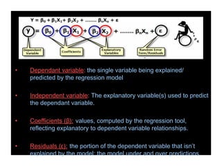
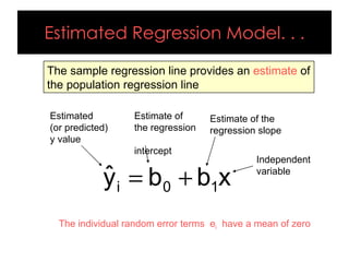
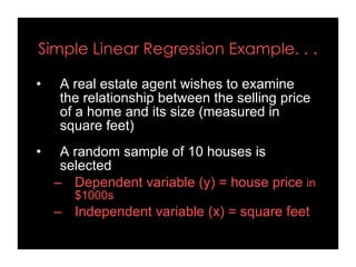
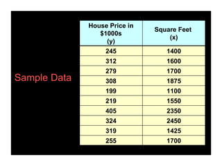
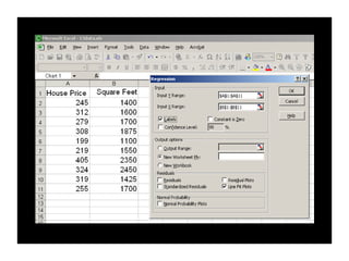
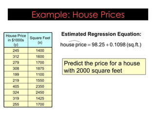
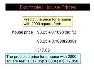
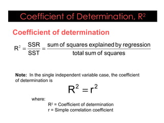
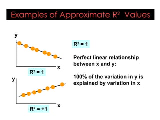
This document provides an overview of regression analysis and its applications in business. It defines regression analysis as the study of relationships between variables, with a dependent variable being explained or predicted by one or more independent variables. Simple linear regression involves one independent variable, while multiple regression can include any number. The document outlines key regression concepts like coefficients, residuals, and linear vs. nonlinear relationships. It provides an example comparing house prices to square footage to illustrate a simple linear regression model. Key outputs from the regression including the equation, R-squared, standard error, and coefficient significance are also explained.

1. REGRESSION ANALYSIS
M.Ravishankar
[ And it’s application in Business ]

2. Introduction. . .
• Father of Regression Analysis
Carl F. Gauss (1777-1855).
• contributions to physics, Mathematics &
astronomy.
• The term “Regression” was first used in
1877 by Francis Galton.

3. Regression Analysis. . .
• It is the study of the
relationship between
variables.
• It is one of the most
commonly used tools for
business analysis.
• It is easy to use and
applies to many
situations.

4. Regression types. . .
• Simple Regression: single explanatory
variable
• Multiple Regression: includes any number of
explanatory variables.

5. • Dependant variable: the single variable being explained/
predicted by the regression model
• Independent variable: The explanatory variable(s) used to predict
the dependant variable.
• Coefficients (β): values, computed by the regression tool,
reflecting explanatory to dependent variable relationships.
• Residuals (ε): the portion of the dependent variable that isn’t
explained by the model; the model under and over predictions.

6. Regression Analysis. . .
• Linear Regression: straight-line relationship
– Form: y=mx+b
• Non-linear: implies curved relationships
– logarithmic relationships

7. Regression Analysis. . .
• Cross Sectional: data gathered from the
same time period
• Time Series: Involves data observed over
equally spaced points in time.

8. Simple Linear Regression Model. . .
• Only one
independent
variable, x
• Relationship
between x and y
is described by a
linear function
• Changes in y are
assumed to be
caused by changes
in x

9. Types of Regression Models. . .

10. x
b
b
ŷ 1
0
i +
=
The sample regression line provides an estimate of
the population regression line
Estimated Regression Model. . .
Estimate of
the regression
intercept
Estimate of the
regression slope
Estimated
(or predicted)
y value
Independent
variable
The individual random error terms ei have a mean of zero

11. Simple Linear Regression Example. . .
• A real estate agent wishes to examine
the relationship between the selling price
of a home and its size (measured in
square feet)
• A random sample of 10 houses is
selected
– Dependent variable (y) = house price in
$1000s
– Independent variable (x) = square feet

12. Sample Data
House Price in
$1000s
(y)
Square Feet
(x)
245 1400
312 1600
279 1700
308 1875
199 1100
219 1550
405 2350
324 2450
319 1425
255 1700

14. Output. . .
Regression Statistics
Multiple R 0.76211
R Square 0.58082
Adjusted R
Square 0.52842
Standard Error 41.33032
Observations 10
ANOVA
df SS MS F
Significance
F
Regression 1 18934.9348 18934.9348 11.0848 0.01039
Residual 8 13665.5652 1708.1957
Total 9 32600.5000
Coefficient
s Standard Error t Stat P-value Lower 95%
Upper
95%
Intercept 98.24833 58.03348 1.69296 0.12892 -35.57720 232.07386
Square Feet 0.10977 0.03297 3.32938 0.01039 0.03374 0.18580
The regression equation is:
feet)
(square
0.10977
98.24833
price
house +
=

15. 0
50
100
150
200
250
300
350
400
450
0 500 1000 1500 2000 2500 3000
Square Feet
House
Price
($1000s)
Graphical Presentation . . .
• House price model: scatter plot and
regression line
feet)
(square
0.10977
98.24833
price
house +
=
Slope
= 0.10977
Intercept
= 98.248

16. Interpretation of the Intercept, b0
• b0 is the estimated average value of Y when the
value of X is zero (if x = 0 is in the range of
observed x values)
– Here, no houses had 0 square feet, so b0 = 98.24833
just indicates that, for houses within the range of sizes
observed, $98,248.33 is the portion of the house price
not explained by square feet
feet)
(square
0.10977
98.24833
price
house +
=

17. Interpretation of the Slope Coefficient, b1
• b1 measures the estimated change in the
average value of Y as a result of a one-
unit change in X
– Here, b1 = .10977 tells us that the average value of a
house increases by .10977($1000) = $109.77, on
average, for each additional one square foot of size
feet)
(square
0.10977
98.24833
price
house +
=

18. House Price
in $1000s
(y)
Square Feet
(x)
245 1400
312 1600
279 1700
308 1875
199 1100
219 1550
405 2350
324 2450
319 1425
255 1700
(sq.ft.)
0.1098
98.25
price
house +
=
Estimated Regression Equation:
Example: House Prices
Predict the price for a house
with 2000 square feet

19. 317.85
0)
0.1098(200
98.25
(sq.ft.)
0.1098
98.25
price
house
=
+
=
+
=
Example: House Prices
Predict the price for a house
with 2000 square feet:
The predicted price for a house with 2000
square feet is 317.85($1,000s) = $317,850

20. Coefficient of determination
Coefficient of Determination, R2
squares
of
sum
total
regression
by
explained
squares
of
sum
SST
SSR
R =
=
2
Note: In the single independent variable case, the coefficient
of determination is
where:
R2
= Coefficient of determination
r = Simple correlation coefficient
2
2
r
R =

21. R2
= +1
Examples of Approximate R2
Values
y
x
y
x
R2
= 1
R2
= 1
Perfect linear relationship
between x and y:
100% of the variation in y is
explained by variation in x

22. Examples of Approximate R2
Values
y
x
y
x
0 < R2
< 1
Weaker linear relationship
between x and y:
Some but not all of the
variation in y is explained
by variation in x

23. Examples of Approximate R2
Values
R2
= 0
No linear relationship
between x and y:
The value of Y does not
depend on x. (None of the
variation in y is explained
by variation in x)
y
x
R2
= 0

24. Output. . .
Regression Statistics
Multiple R 0.76211
R Square 0.58082
Adjusted R
Square 0.52842
Standard Error 41.33032
Observations 10
ANOVA
df SS MS F
Significance
F
Regression 1 18934.9348
18934.934
8
11.084
8 0.01039
Residual 8 13665.5652 1708.1957
Total 9 32600.5000
Coefficien
ts Standard Error t Stat
P-
value Lower 95%
Upper
95%
0.1289 232.0738
58.08%
58.08% of the variation in
house prices is explained by
variation in square feet
0.58082
32600.5000
18934.9348
SST
SSR
R2
=
=
=

25. Standard Error of Estimate. . .
• The standard deviation of the variation of
observations around the regression line is
estimated by
1
−
−
=
ε
k
n
SSE
s
Where
SSE = Sum of squares error
n = Sample size
k = number of independent variables in the
model

26. The Standard Deviation of the
Regression Slope
• The standard error of the regression slope
coefficient (b1) is estimated by
∑ ∑
∑ −
=
−
=
n
x)
(
x
s
)
x
(x
s
s
2
2
ε
2
ε
b1
where:
= Estimate of the standard error of the least squares slope
= Sample standard error of the estimate
1
b
s
2
n
SSE
sε
−
=

27. Output. . .
Regression Statistics
Multiple R 0.76211
R Square 0.58082
Adjusted R
Square 0.52842
Standard Error 41.33032
Observations 10
ANOVA
df SS MS F
Significance
F
Regression 1 18934.9348
18934.934
8
11.084
8 0.01039
Residual 8 13665.5652 1708.1957
Total 9 32600.5000
Coefficien
ts Standard Error t Stat
P-
value Lower 95%
Upper
95%
0.1289 232.0738
41.33032
sε =
0.03297
s 1
b =

28. Reference. . .
• Business
Business statistics by S.P.Gupta & M.P.Gupta
Sources retrieved from Internet…
• www.humboldt.edu
• www.cs.usask.ca
• www.cab.latech.edu
• www.quickmba.com
• www.wikipedia.com
• www.youtube.com

29. M.RAVISHANKAR
MBA(AB) 2008-2010 Batch
NIFTTEA KNITWEAR FASHION
INSTITUTE
TIRUPUR
OXYGEN024@GMAIL.COM