The document provides an overview of regression analysis, detailing its role in predicting and explaining the relationship between independent and dependent variables. It distinguishes between correlation and regression, highlighting that regression demonstrates cause and effect relationships, whereas correlation does not. An example of simple linear regression is presented, illustrating how to predict house prices based on square footage.

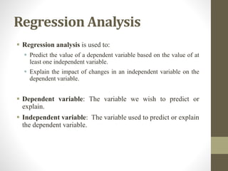
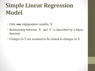
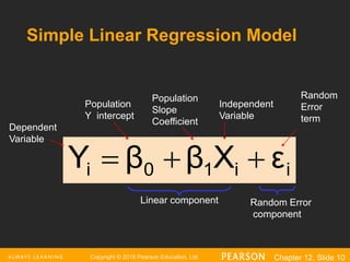
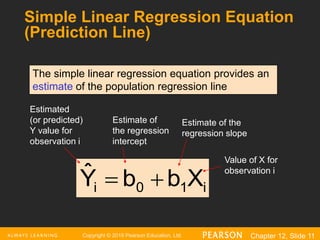
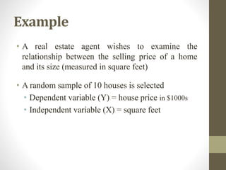
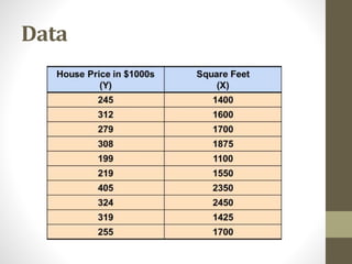
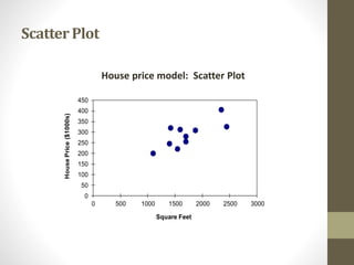
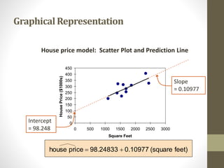
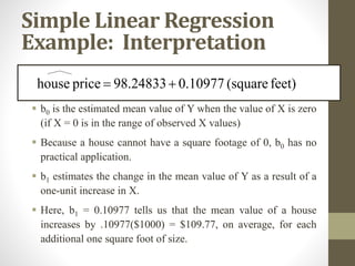
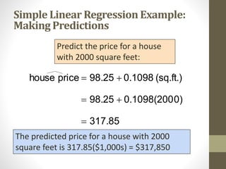
1. REGRESSION
ANALYSIS
Dr.BalamuruganM
AssociateProfessor
AcharyaInstituteofGraduateStudies
Bangalore

2. Regression
• Regression analysis measures the nature and extent of the
relationship between two or more variables, thus enables
us to make predictions.
• Regression is the measure of the average relationship
between two or more variables.

3. Correlation vs. Regression
• Degree & Nature of Relationship
 Correlation is a measure of degree of relationship between X
& Y.
 Regression studies the nature of relationship between the
variables so that one may be able to predict the value of one
variable on the basis of another.
• Cause & Effect Relationship
 Correlation does not assume cause and effect relationship
between two variables.
 Regression clearly expresses the cause and effect relationship
between two variables. The independent variable is the cause
and dependent variable is effect.

4. Correlation vs. Regression
• Prediction
 Correlation does not help in making predictions.
 Regression enable us to make predictions using
regression line.
• Symmetric
 Correlation coefficients are symmetrical.
 Regression coefficients are not symmetrical.

5. Copyright © 2016 Pearson Education, Ltd. Chapter 12, Slide 5
Regression Models
Y
X
Y
X
Y
Y
X
X
Linear relationships Curvilinear relationships

6. Copyright © 2016 Pearson Education, Ltd. Chapter 12, Slide 6
Types of Relationships
Y
X
Y
X
Y
Y
X
X
Strong relationships Weak relationships

7. Copyright © 2016 Pearson Education, Ltd. Chapter 12, Slide 7
Types of Relationships
Y
X
Y
X
No relationship

8. Regression Analysis
 Regression analysis is used to:
 Predict the value of a dependent variable based on the value of at
least one independent variable.
 Explain the impact of changes in an independent variable on the
dependent variable.
 Dependent variable: The variable we wish to predict or
explain.
 Independent variable: The variable used to predict or explain
the dependent variable.

9. Simple Linear Regression
Model
• Only one independent variable, X
• Relationship between X and Y is described by a linear
function
• Changes in Y are assumed to be related to changes in X

10. Copyright © 2016 Pearson Education, Ltd. Chapter 12, Slide 10
i
i
1
0
i ε
X
β
β
Y 


Linear component
Simple Linear Regression Model
Population
Y intercept
Population
Slope
Coefficient
Random
Error
term
Dependent
Variable
Independent
Variable
Random Error
component

11. Copyright © 2016 Pearson Education, Ltd. Chapter 12, Slide 11
Simple Linear Regression Equation
(Prediction Line)
i
1
0
i X
b
b
Ŷ 

The simple linear regression equation provides an
estimate of the population regression line
Estimate of
the regression
intercept
Estimate of the
regression slope
Estimated
(or predicted)
Y value for
observation i
Value of X for
observation i

12. Interpretation of the Slope
and Intercept
• b0 is the estimated mean value of Y when the value of X
is zero.
• b1 is the estimated change in the mean value of Y as a
result of a one-unit increase in X.

13. Example
• A real estate agent wishes to examine the
relationship between the selling price of a home
and its size (measured in square feet)
• A random sample of 10 houses is selected
• Dependent variable (Y) = house price in $1000s
• Independent variable (X) = square feet

14. Data

15. 0
50
100
150
200
250
300
350
400
450
0 500 1000 1500 2000 2500 3000
House
Price
($1000s)
Square Feet
ScatterPlot
House price model: Scatter Plot

16. 0
50
100
150
200
250
300
350
400
450
0 500 1000 1500 2000 2500 3000
Square Feet
House
Price
($1000s)
GraphicalRepresentation
House price model: Scatter Plot and Prediction Line
feet)
(square
0.10977
98.24833
price
house 

Slope
= 0.10977
Intercept
= 98.248

17. Simple Linear Regression
Example: Interpretation
 b0 is the estimated mean value of Y when the value of X is zero
(if X = 0 is in the range of observed X values)
 Because a house cannot have a square footage of 0, b0 has no
practical application.
 b1 estimates the change in the mean value of Y as a result of a
one-unit increase in X.
 Here, b1 = 0.10977 tells us that the mean value of a house
increases by .10977($1000) = $109.77, on average, for each
additional one square foot of size.
feet)
(square
0.10977
98.24833
price
house 


18. 317.85
0)
0.1098(200
98.25
(sq.ft.)
0.1098
98.25
price
house





Predict the price for a house
with 2000 square feet:
The predicted price for a house with 2000
square feet is 317.85($1,000s) = $317,850
Simple Linear Regression Example:
Making Predictions

19. THANK YOU