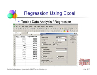
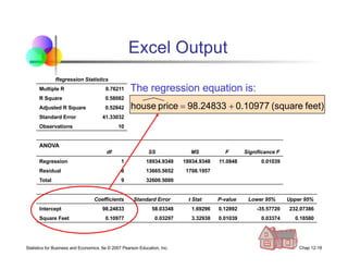
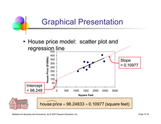
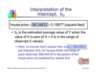
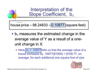
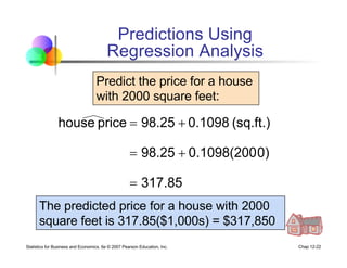
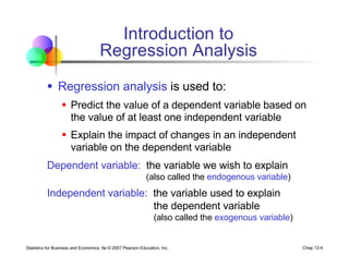
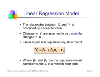
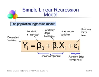
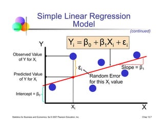
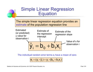
This document discusses simple linear regression analysis. It begins by explaining correlation analysis and how regression analysis is used to predict a dependent variable from independent variables. A linear regression model is presented that estimates the dependent variable (Y) as a linear function of the independent variable (X) plus an error term. The least squares method is described for estimating the slope and intercept coefficients in the regression equation to minimize error. An example using house price data is presented to illustrate finding the regression equation and using it to interpret the slope and intercept as well as make predictions.
![Statistics for Business and Economics, 6e © 2007 Pearson Education, Inc. Chap 12-9
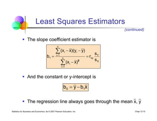
Least Squares Estimators
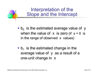
§ b0 and b1 are obtained by finding the values
of b0 and b1 that minimize the sum of the
squared differences between y and :
2
i
1
0
i
2
i
i
2
i
)]
x
b
(b
[y
min
)
y
(y
min
e
min
SSE
min
+
-
=
-
=
=
å
å
å
ˆ
ŷ
Differential calculus is used to obtain the
coefficient estimators b0 and b1 that minimize SSE](https://image.slidesharecdn.com/simpleregression-1-230513173309-175a524e/85/simple-regression-1-pdf-9-320.jpg)
![Statistics for Business and Economics, 6e © 2007 Pearson Education, Inc. Chap 12-12
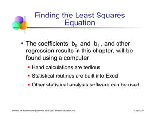
Linear Regression Model
Assumptions
§ The true relationship form is linear (Y is a linear function
of X, plus random error)
§ The error terms, εi are independent of the x values
§ The error terms are random variables with mean 0 and
constant variance, σ2
(the constant variance property is called homoscedasticity)
§ The random error terms, εi, are not correlated with one
another, so that
n)
,
1,
(i
for
σ
]
E[ε
and
0
]
E[ε 2
2
i
i !
=
=
=
j
i
all
for
0
]
ε
E[ε j
i ¹
=](https://image.slidesharecdn.com/simpleregression-1-230513173309-175a524e/85/simple-regression-1-pdf-12-320.jpg)