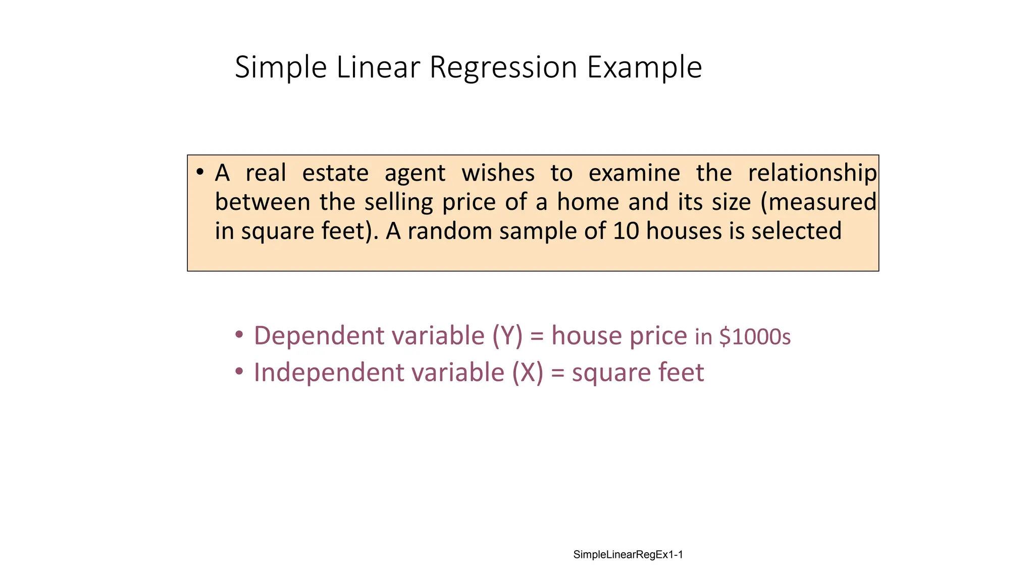
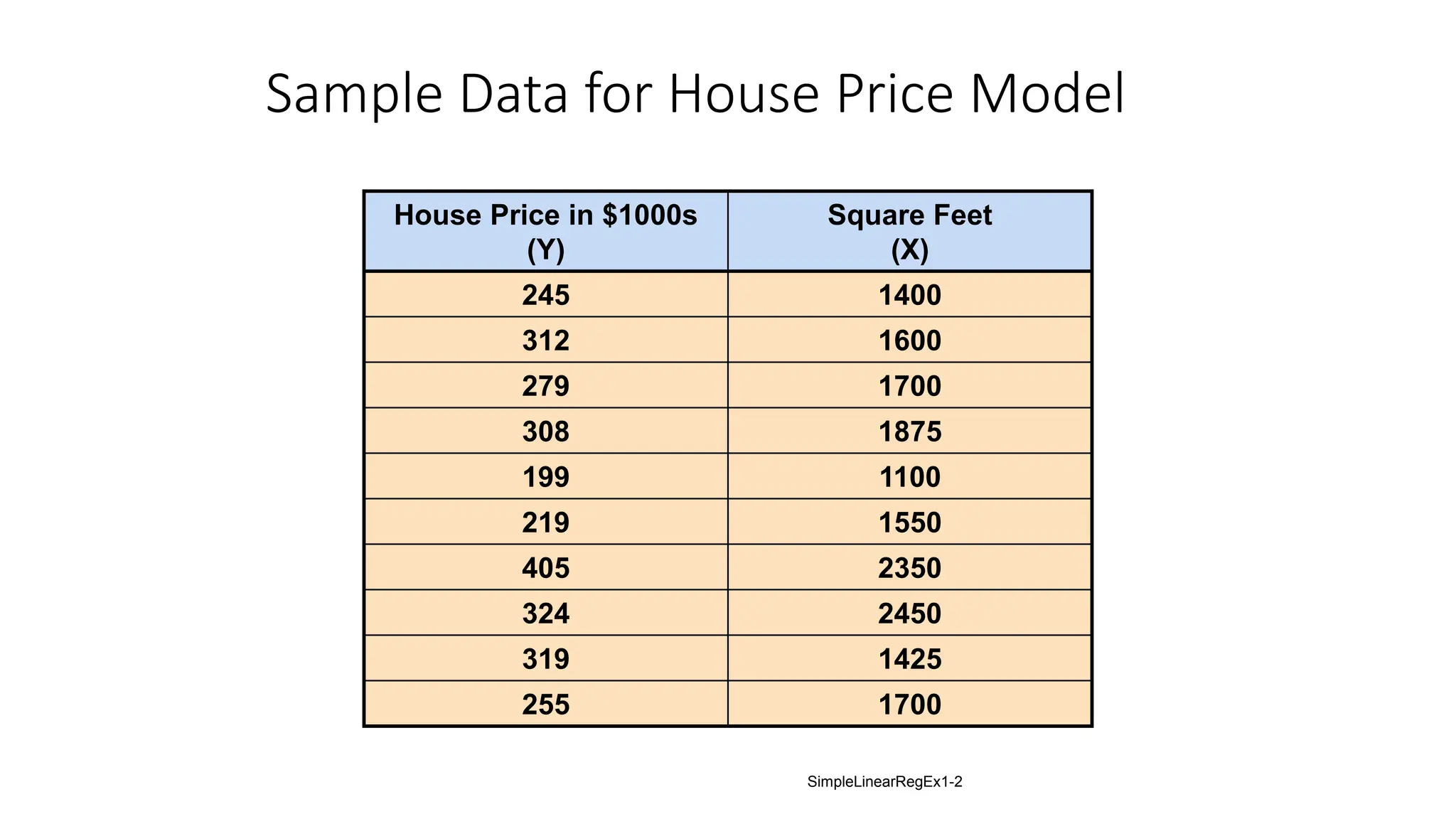
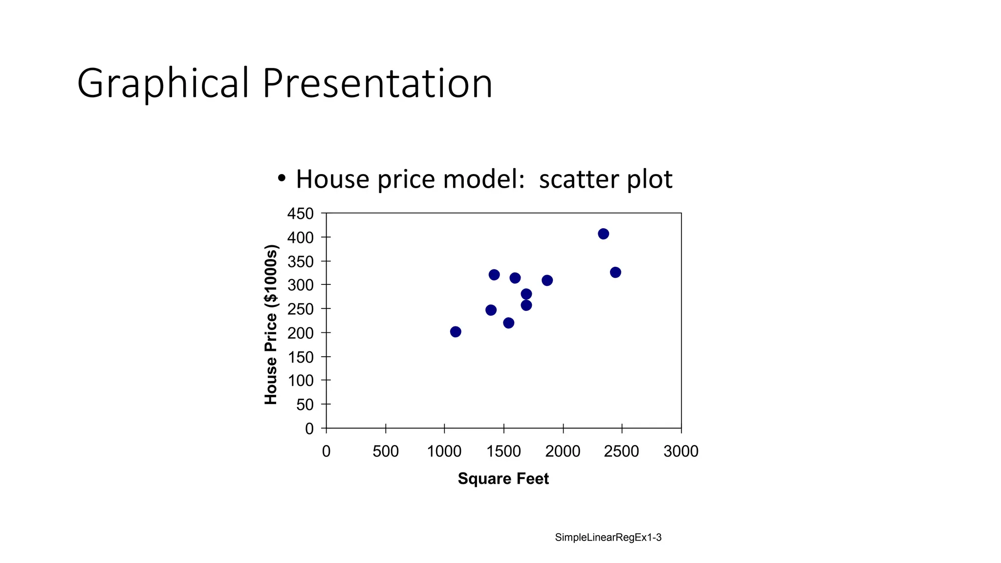
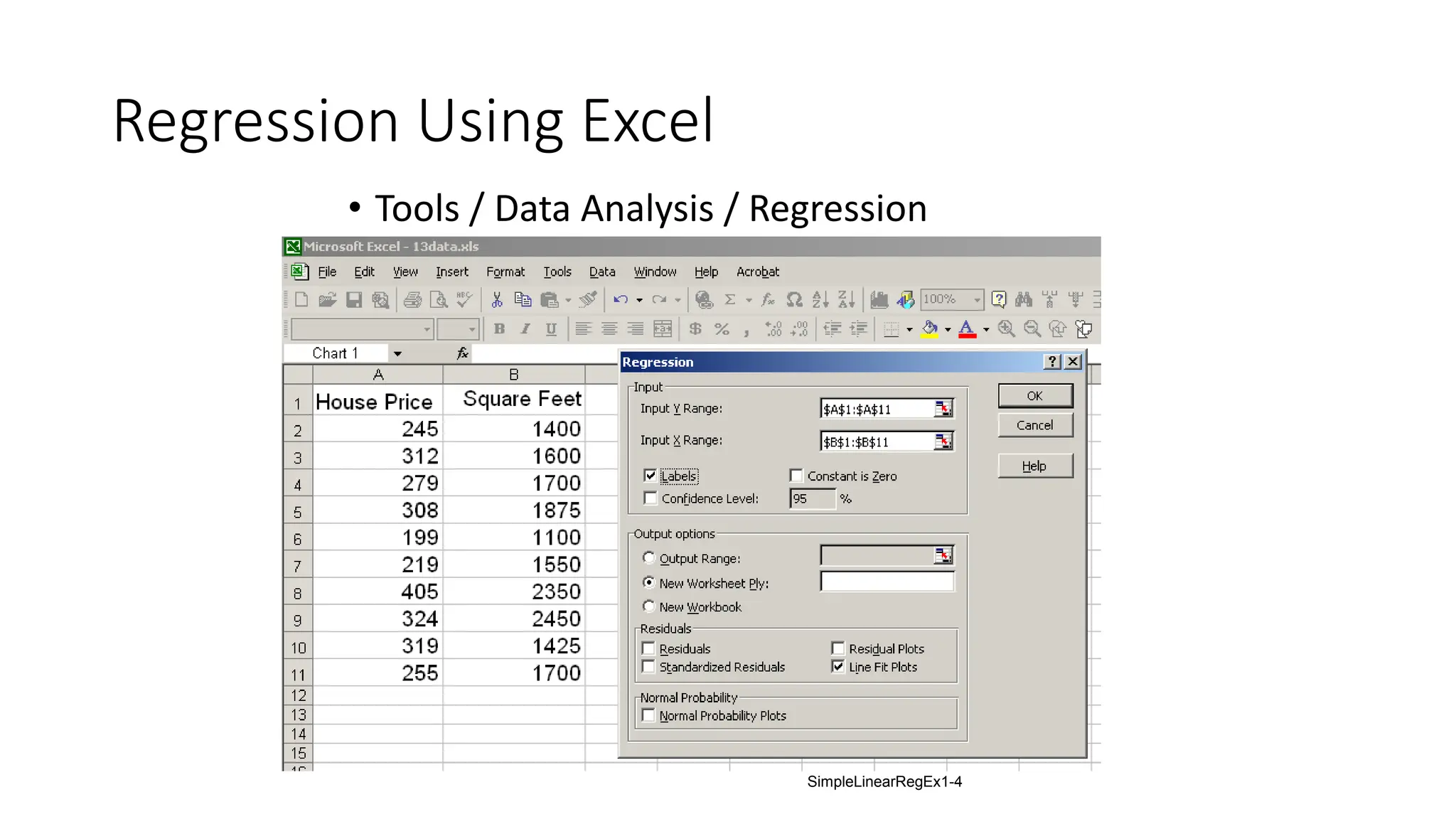
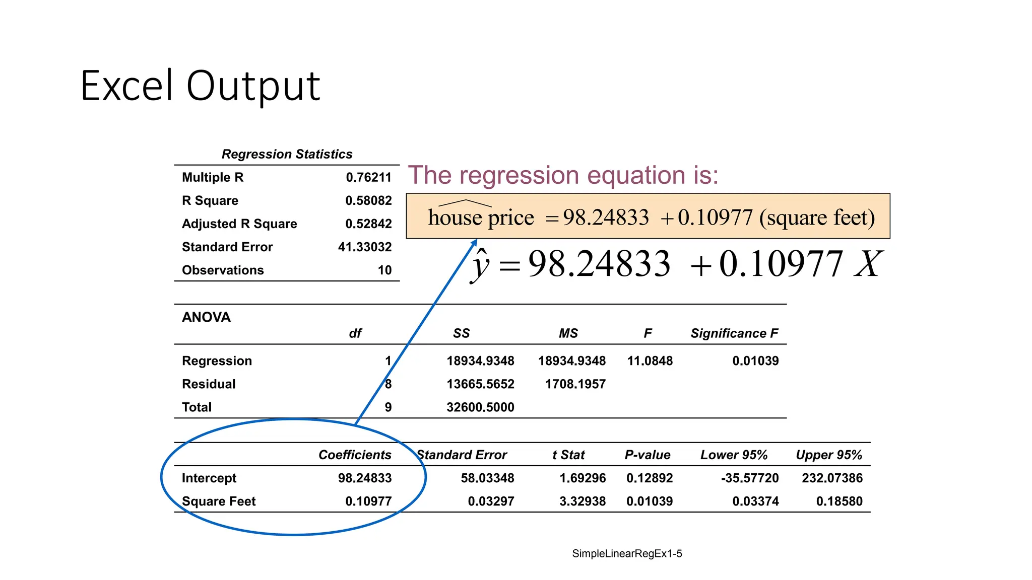
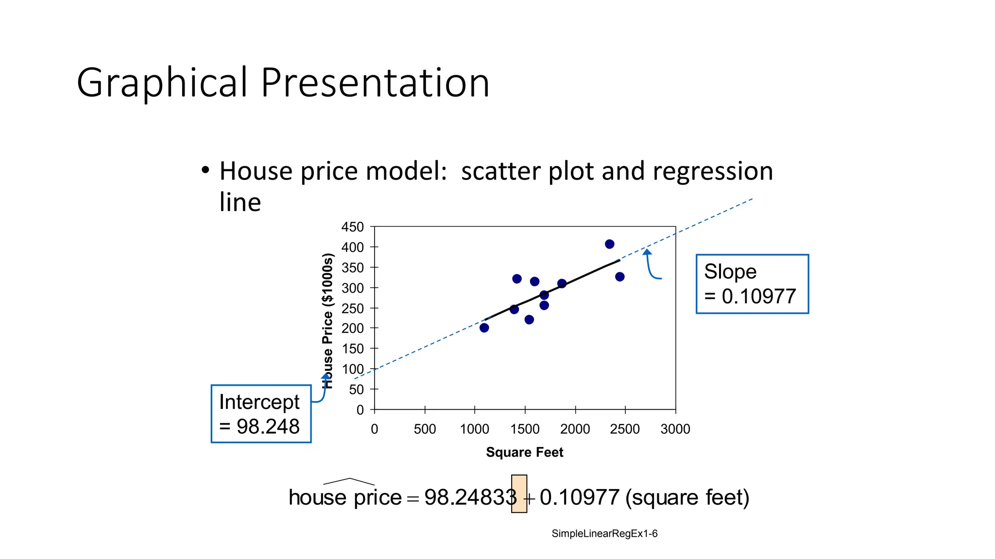
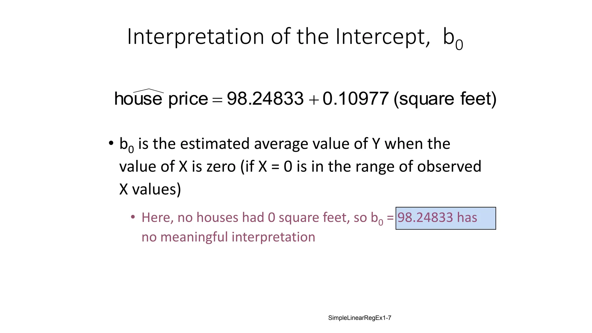
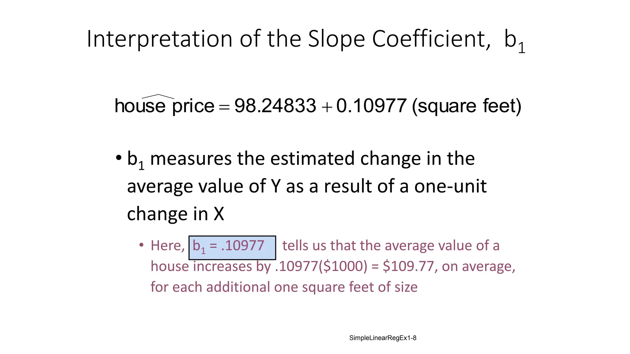
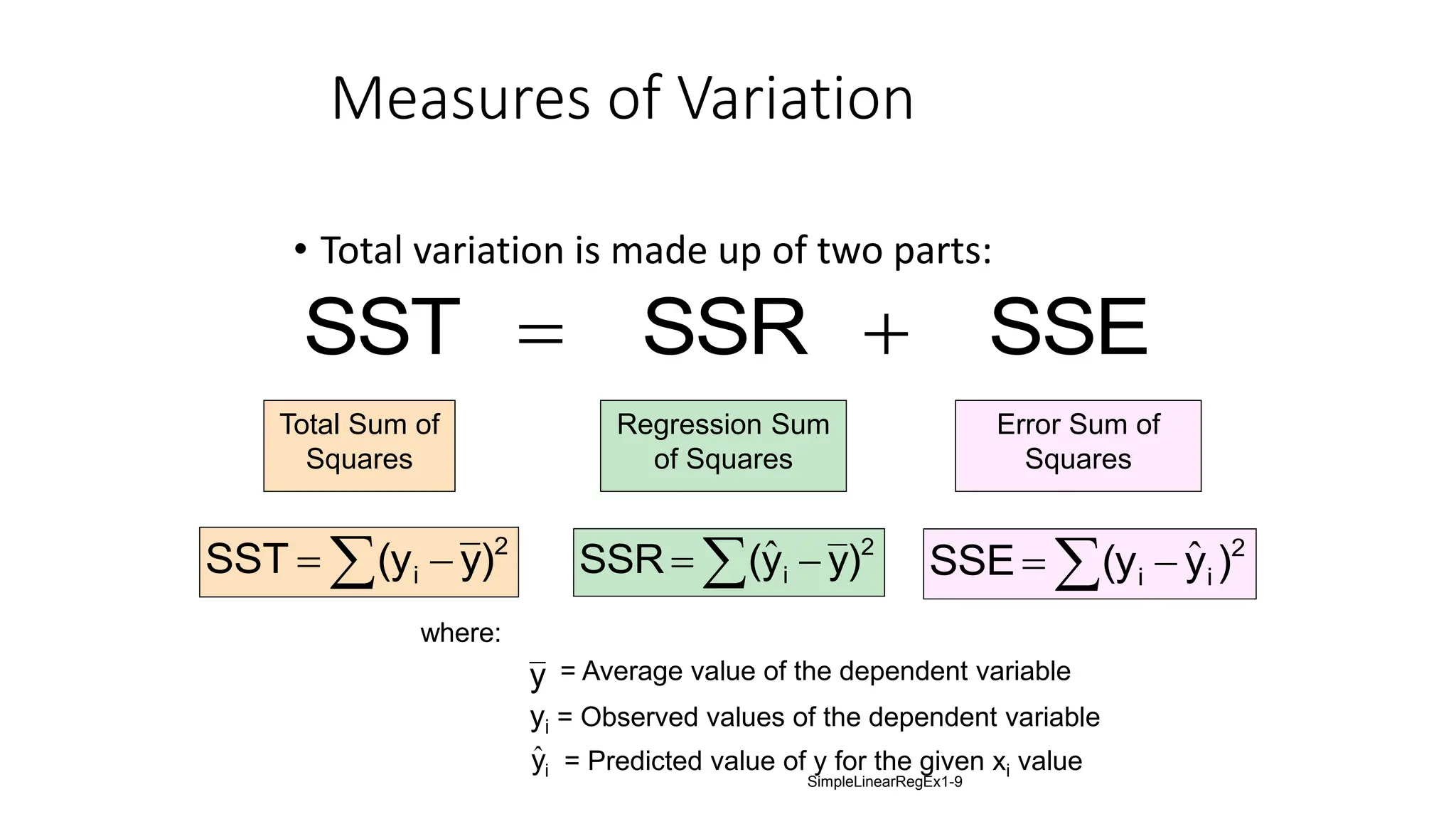
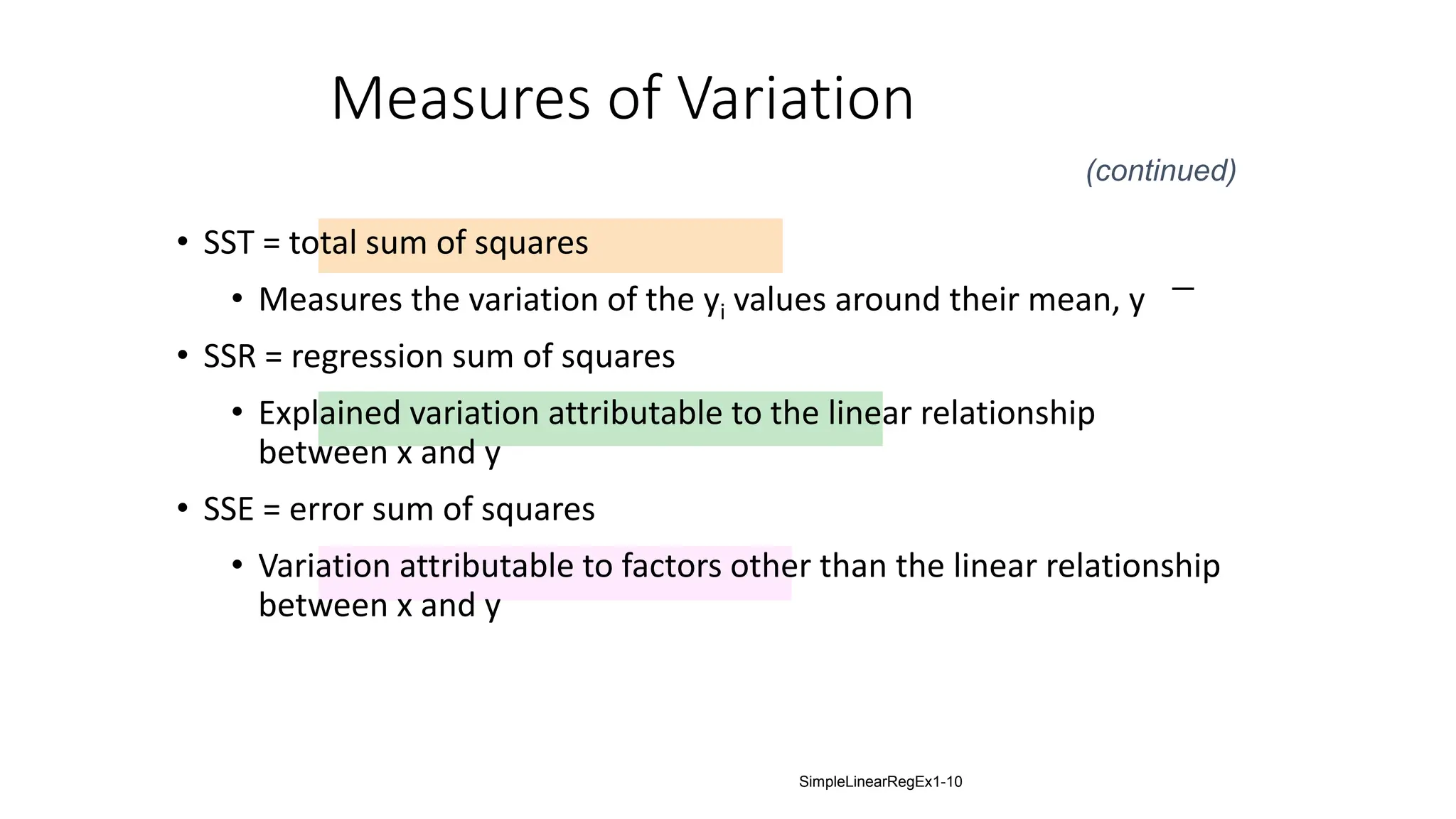
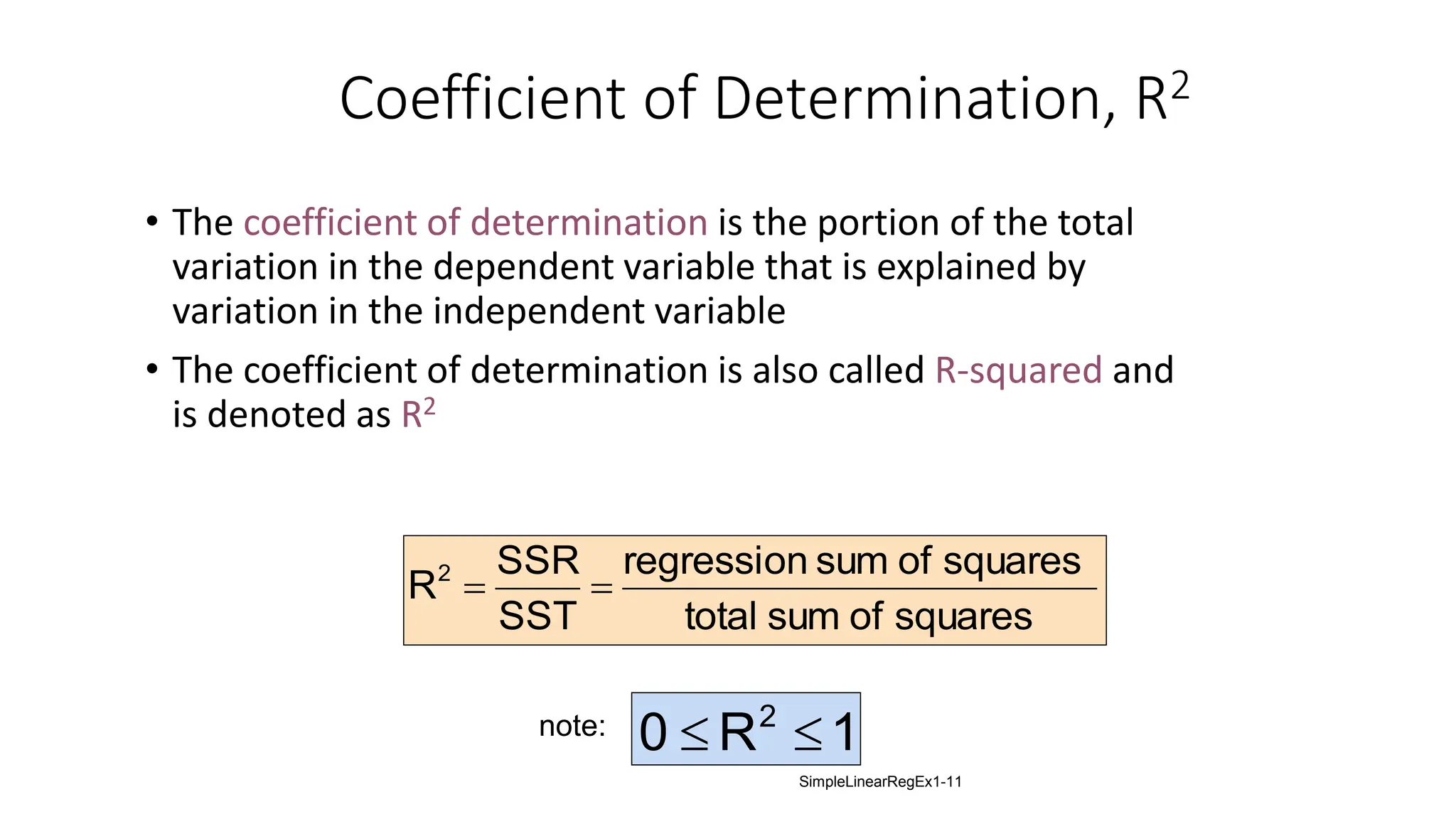
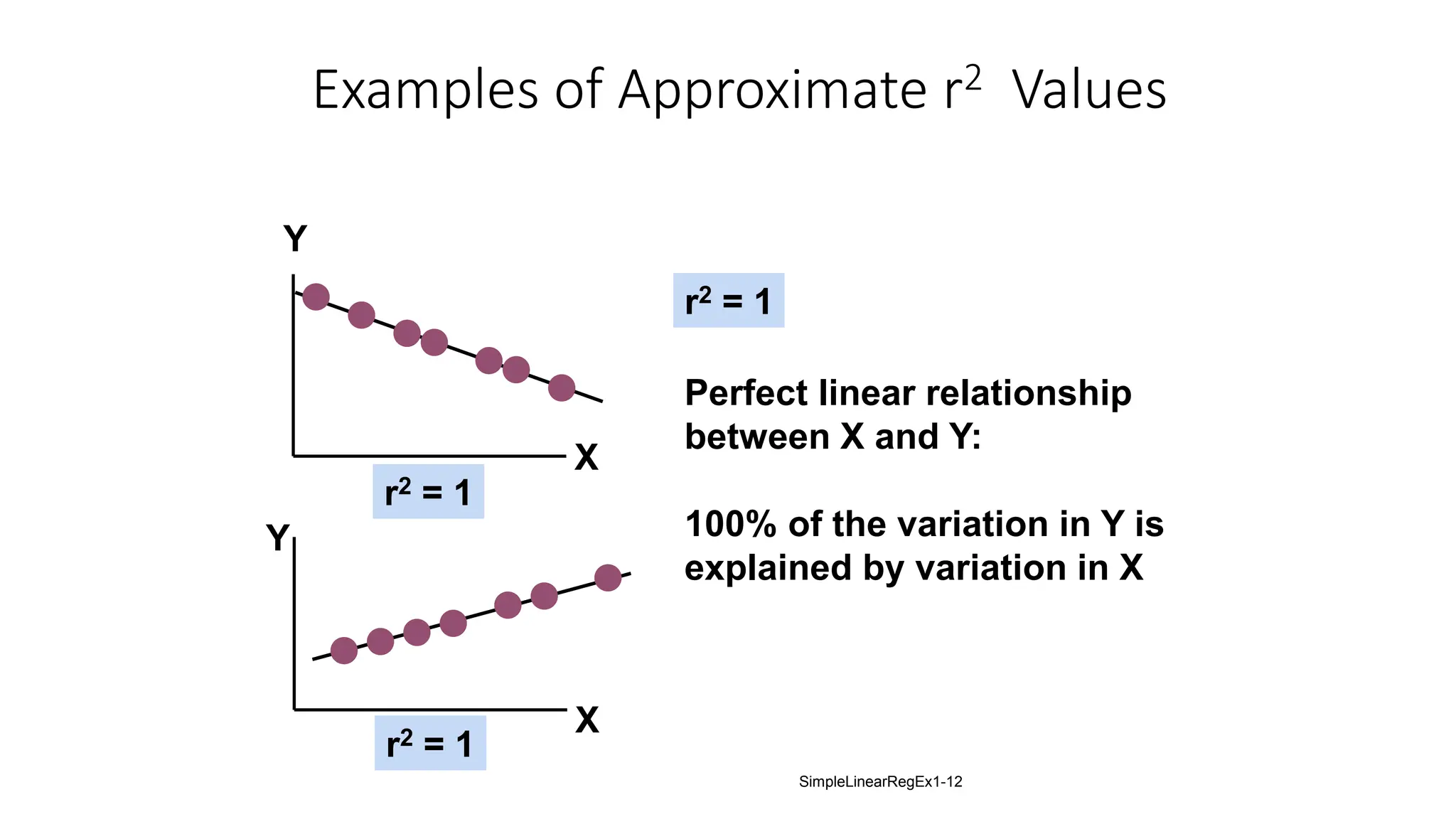
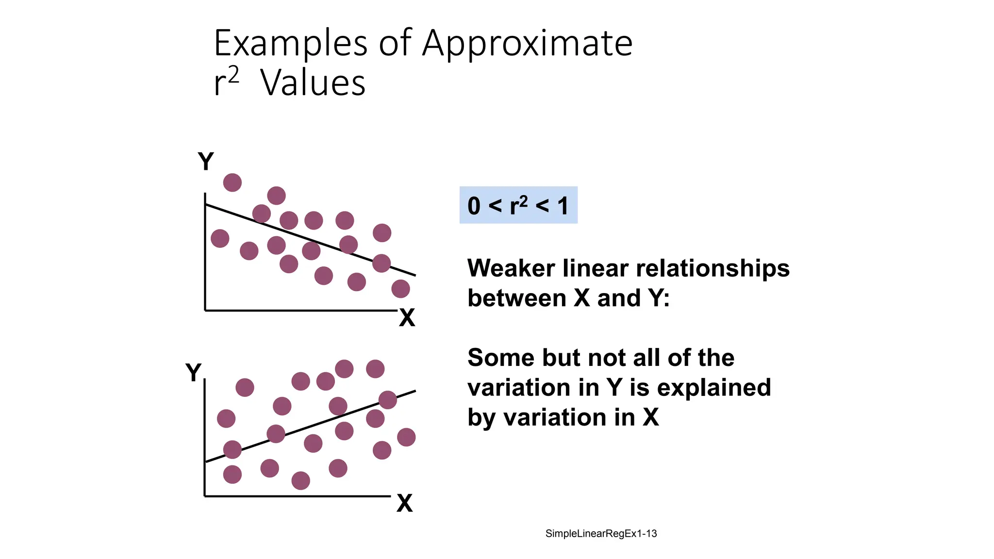
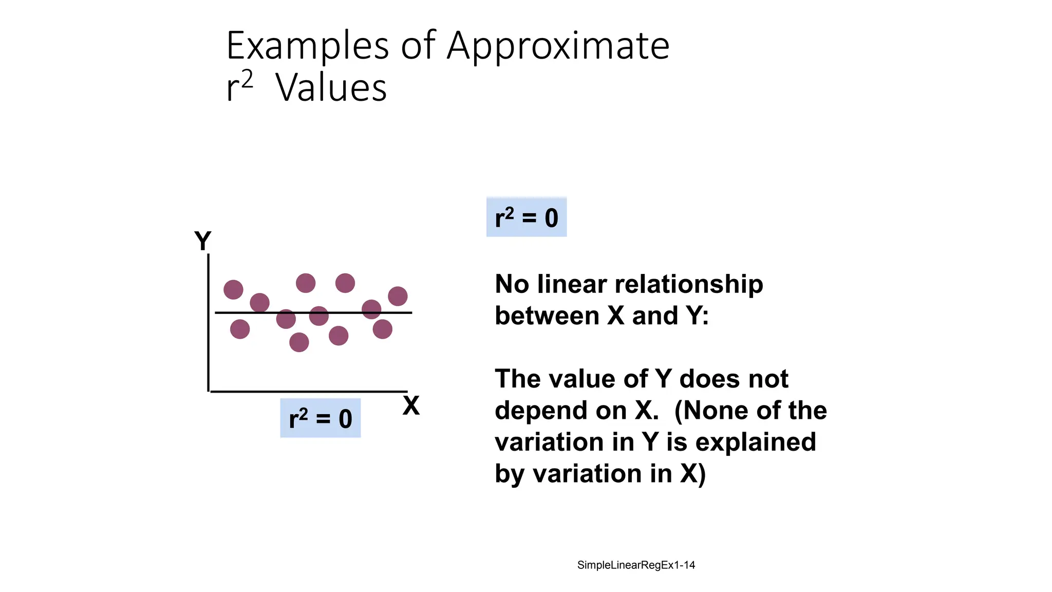
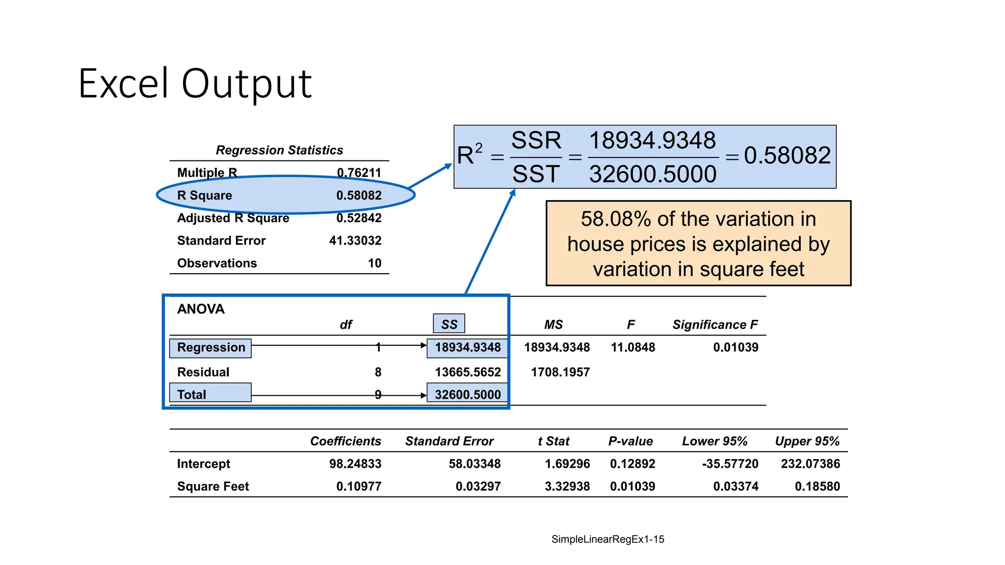
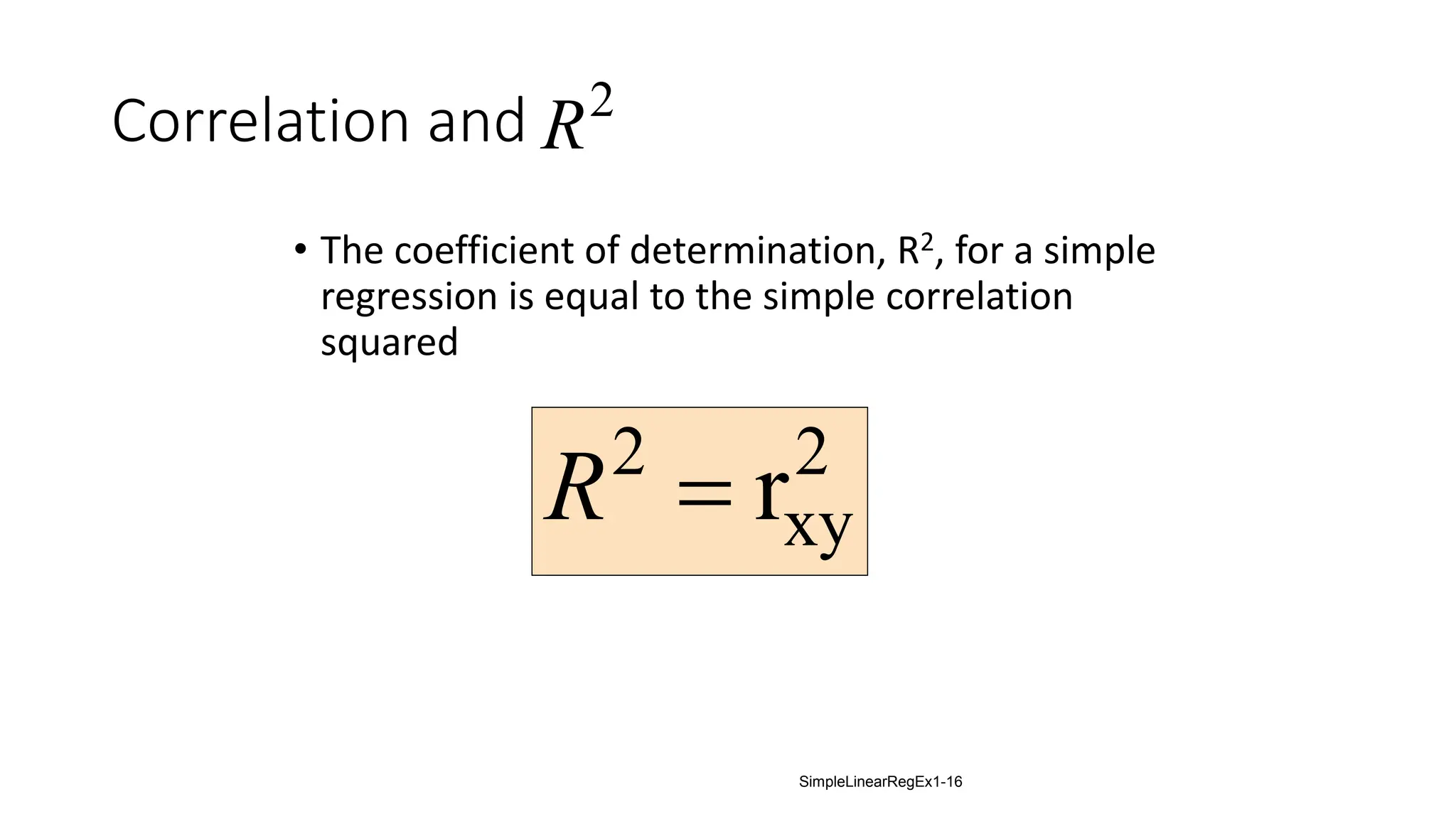
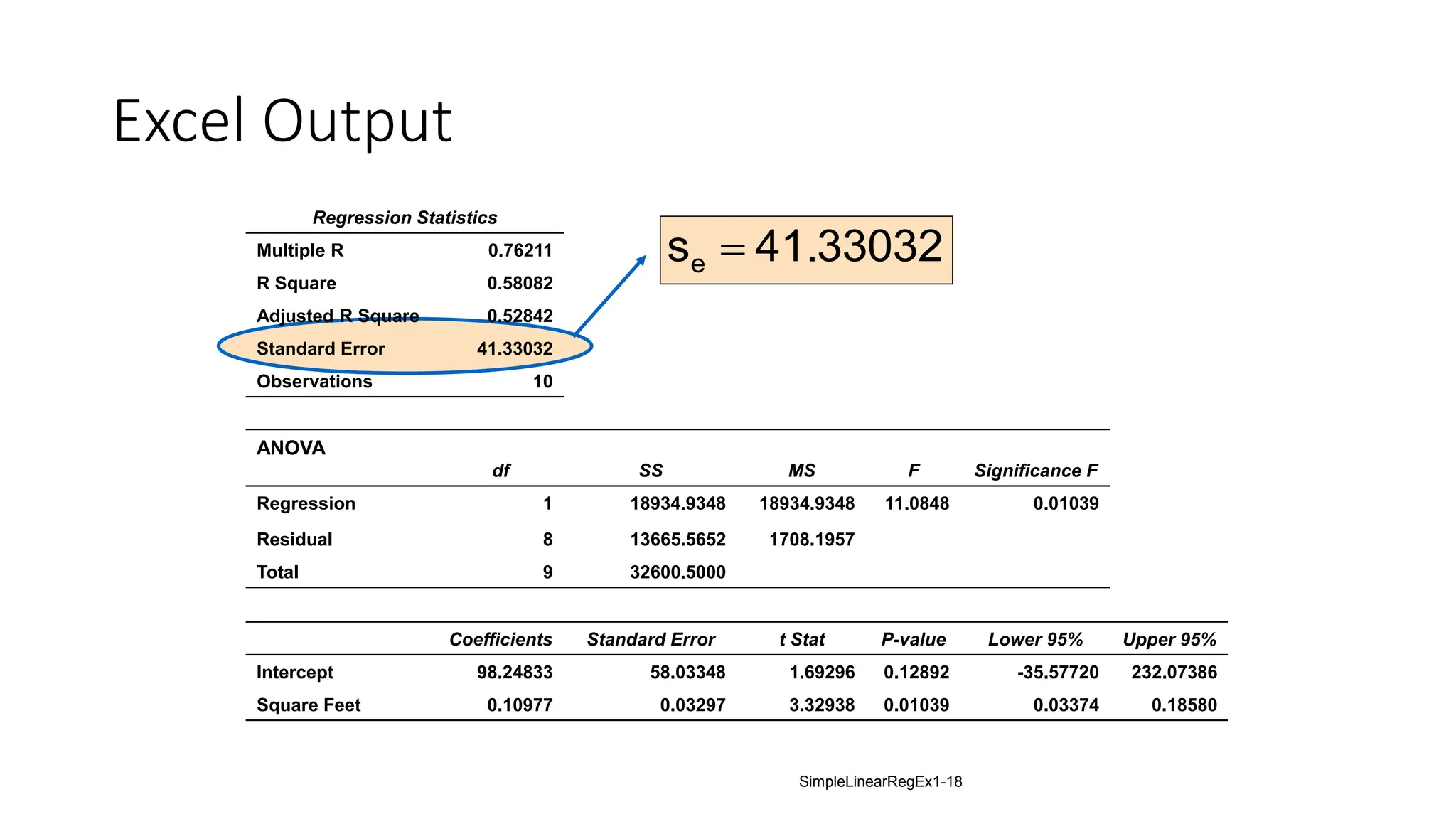
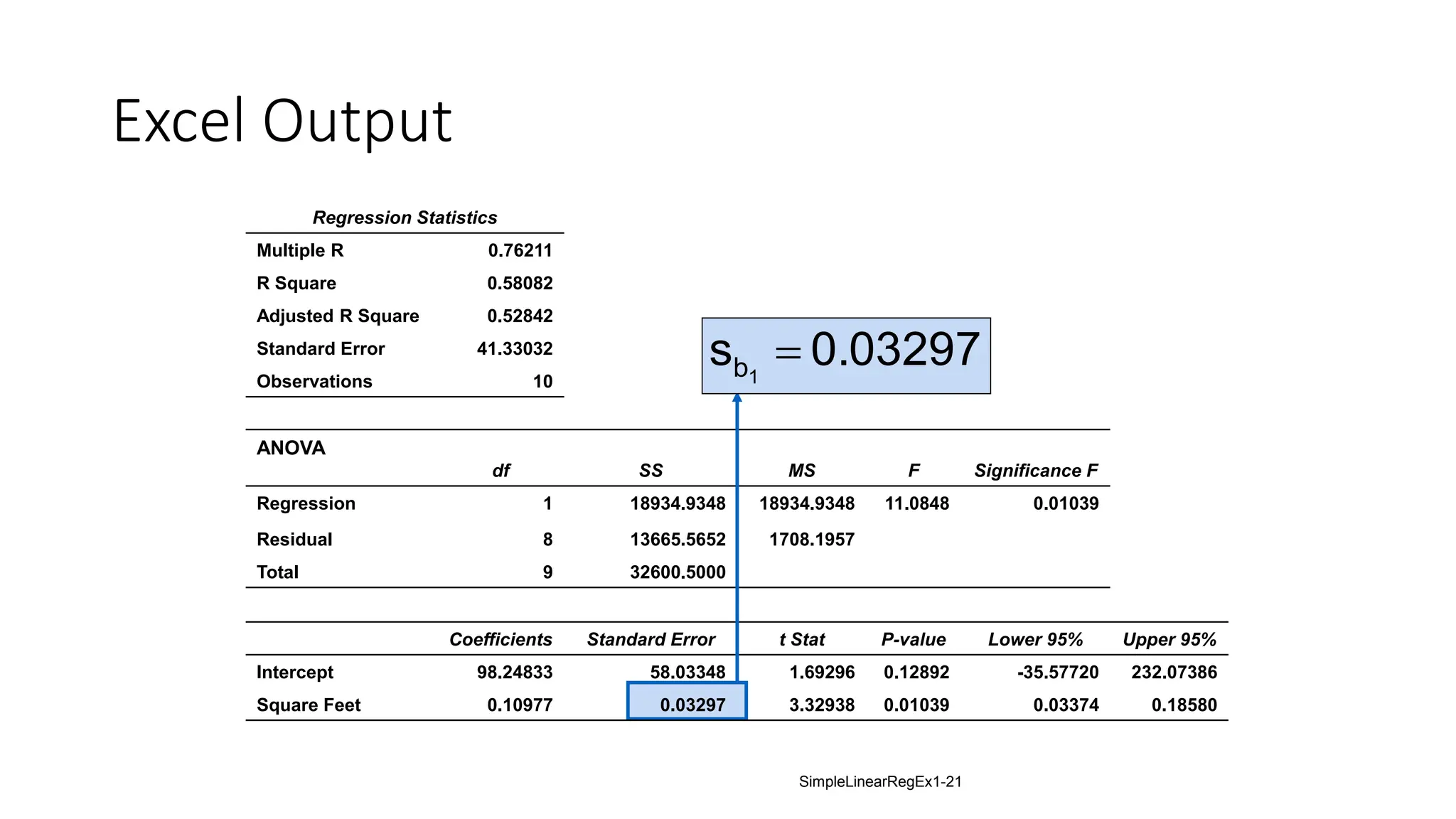
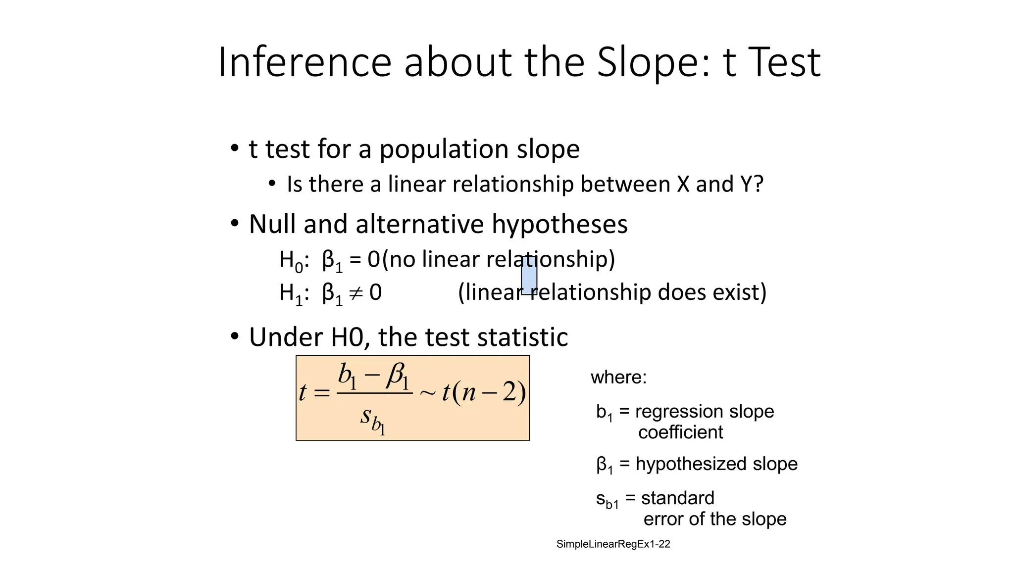
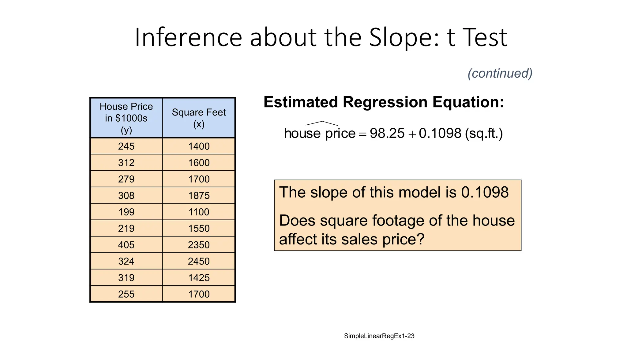
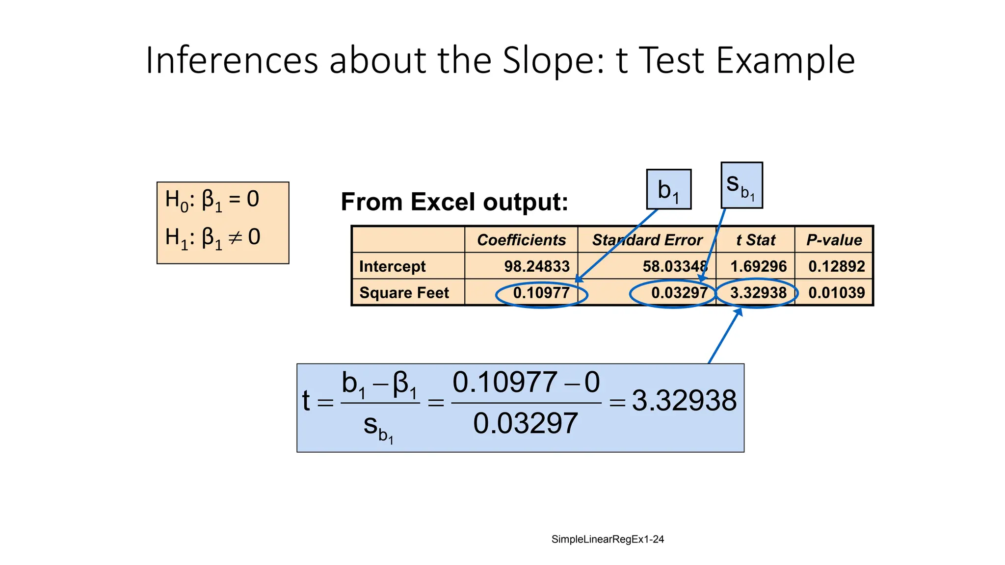
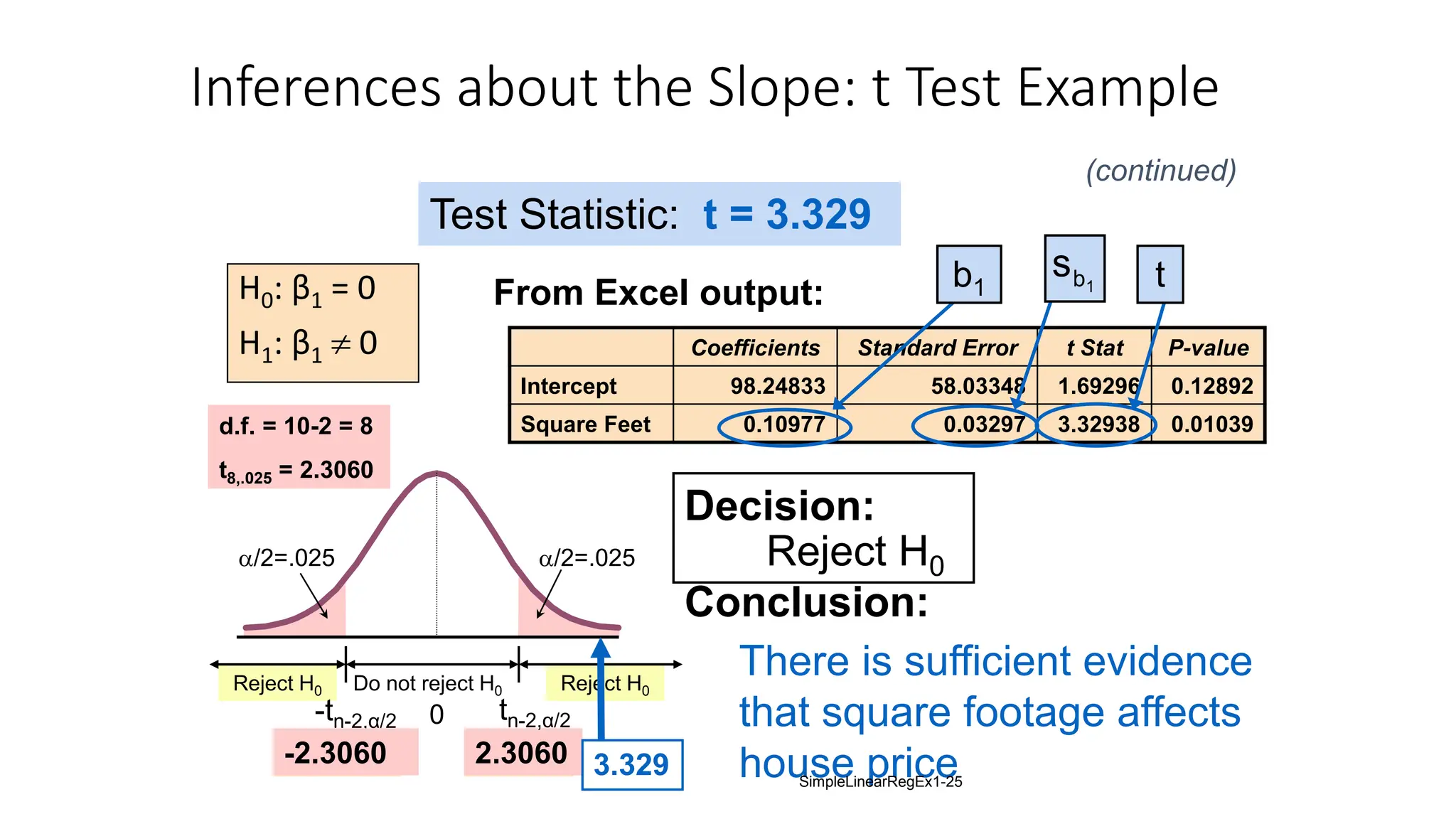
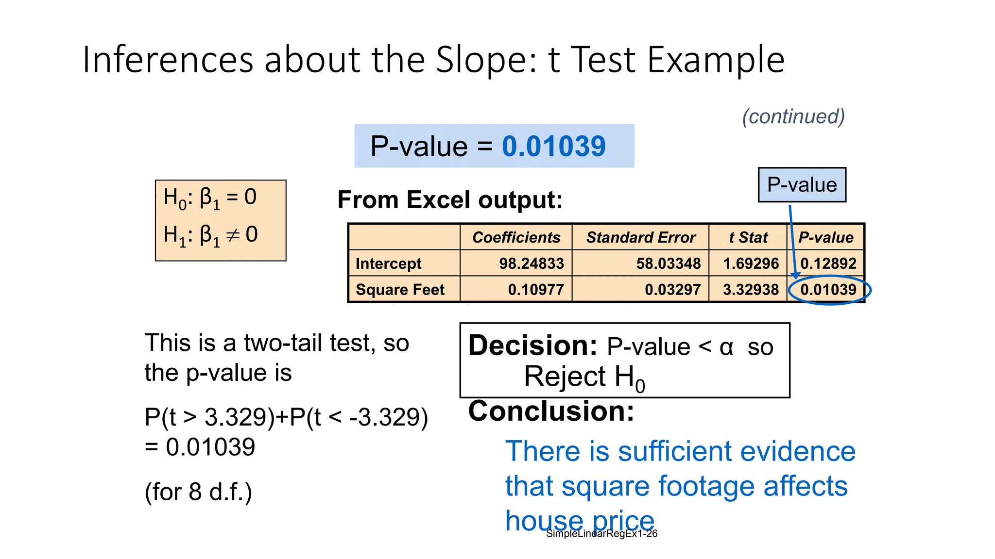
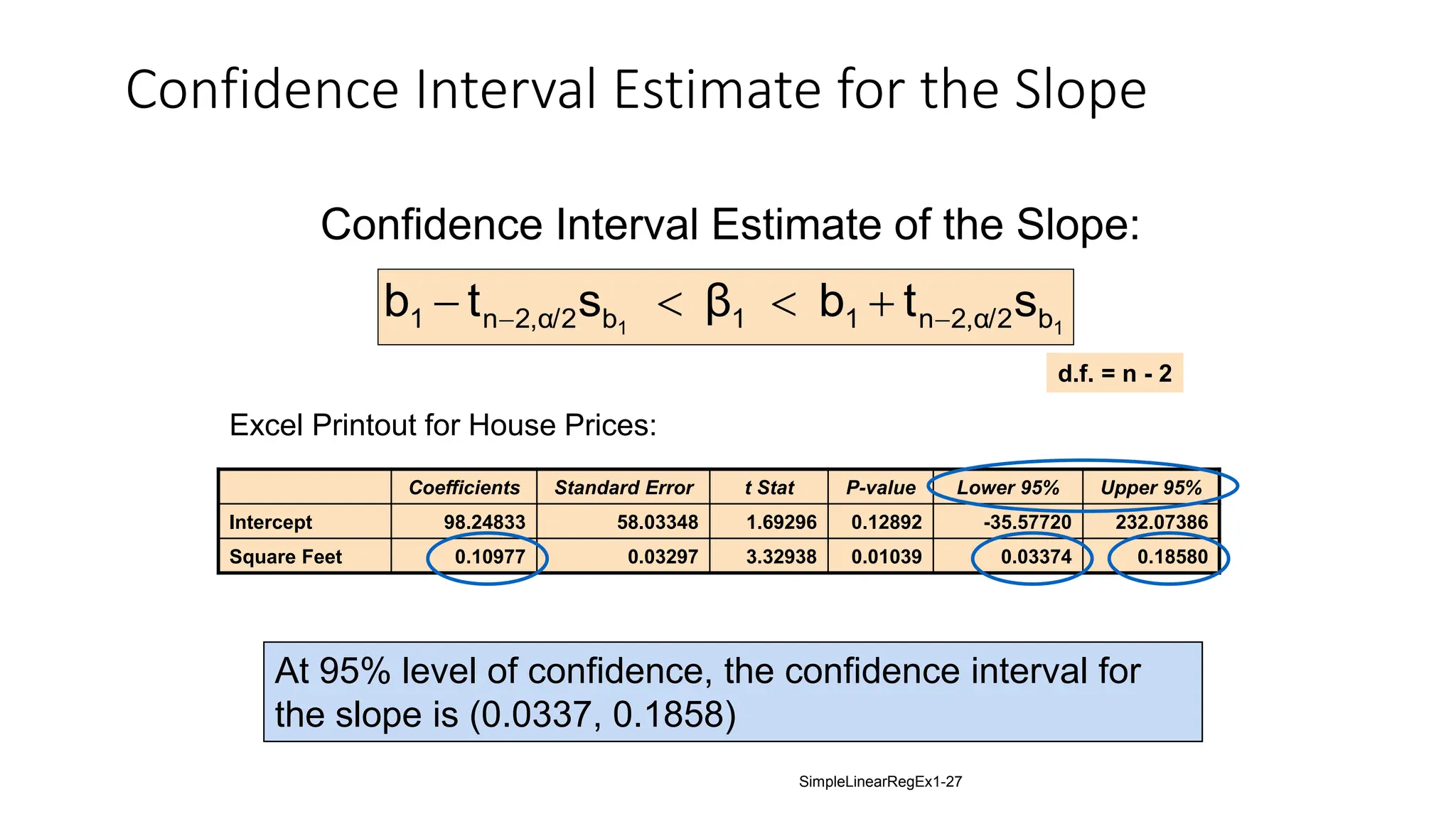
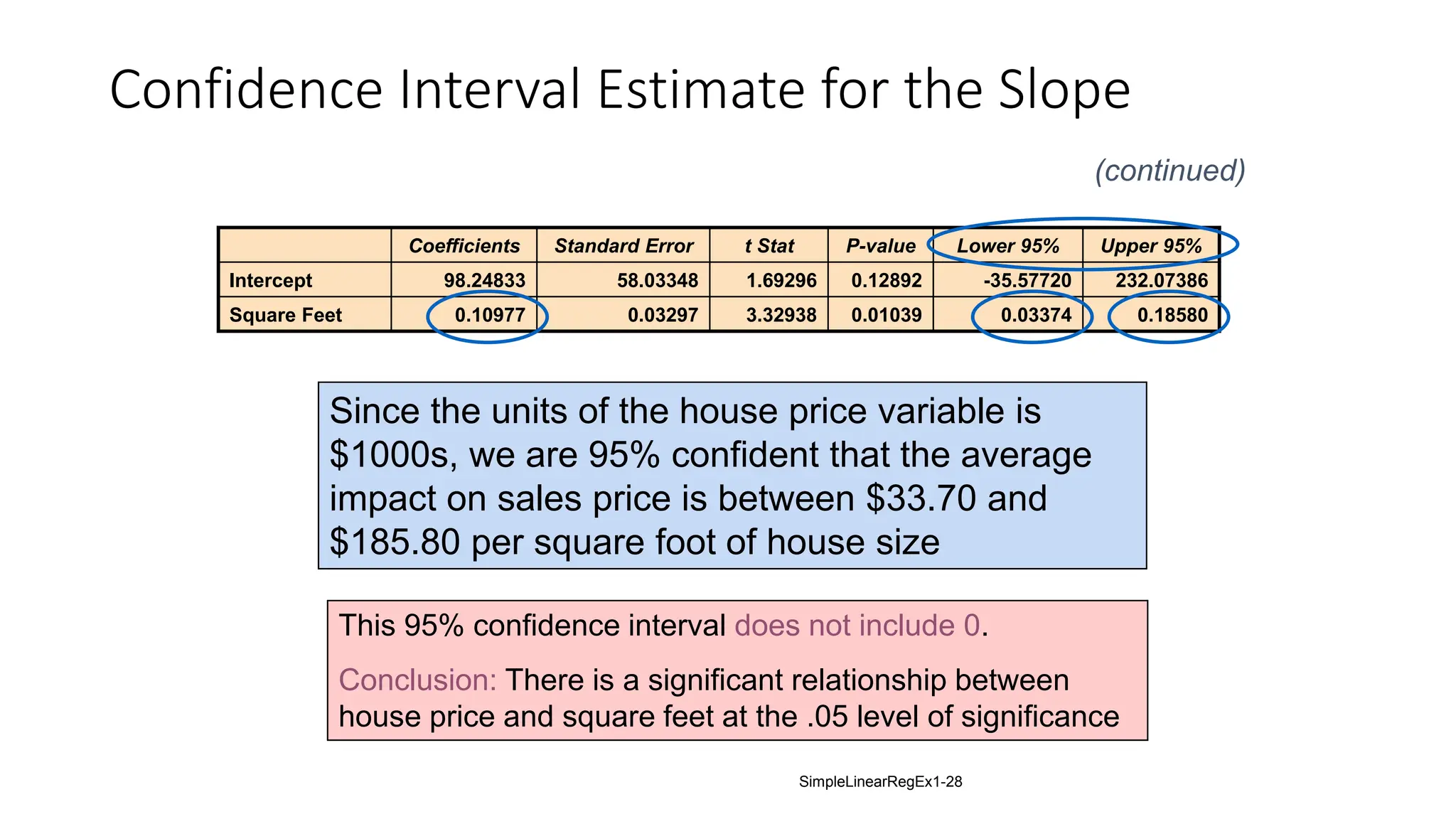
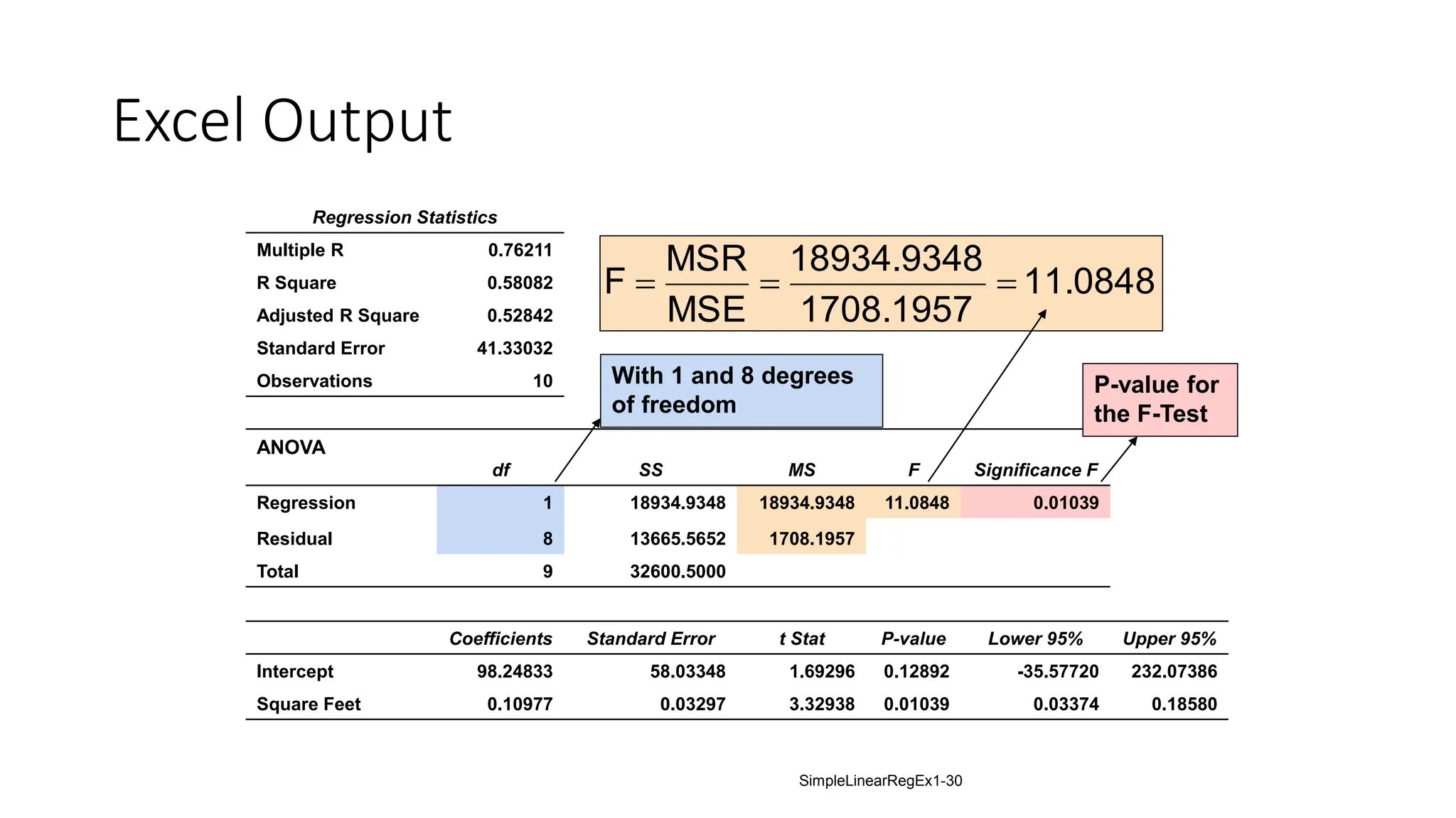
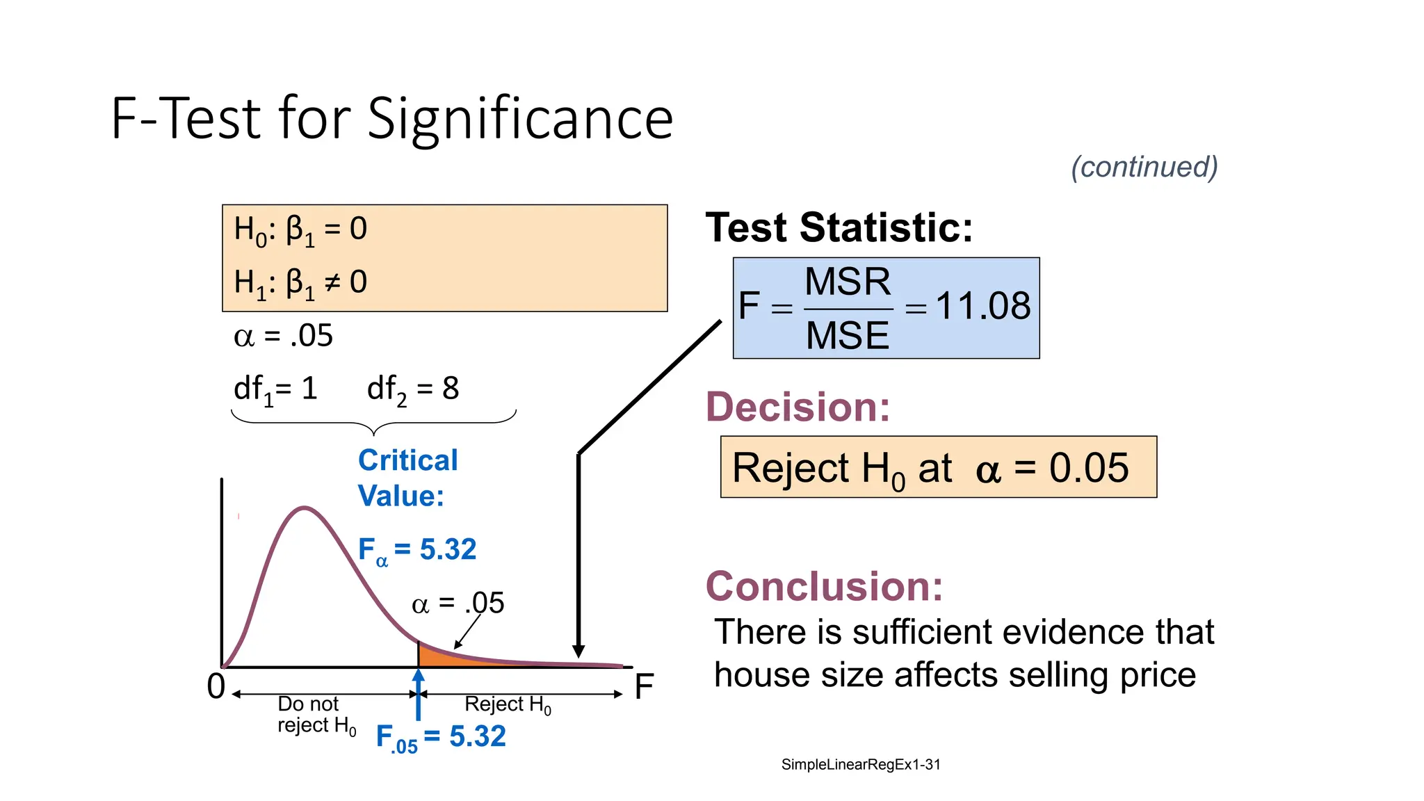
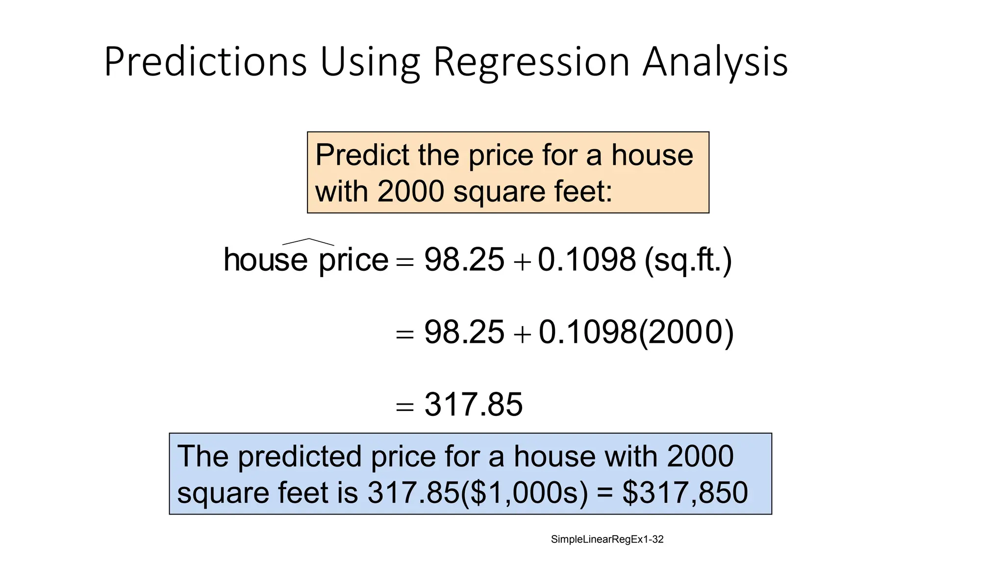
Simple Linear Regression Example
• A real estate agent wishes to examine the relationship
between the selling price of a home and its size (measured
in square feet). A random sample of 10 houses is selected
• Dependent variable (Y) = house price in $1000s
• Independent variable (X) = square feet
SimpleLinearRegEx1-1
Sample Data for House Price Model
House Price in $1000s
(Y)
Square Feet
(X)
245 1400
312 1600
279 1700
308 1875
199 1100
219 1550
405 2350
324 2450
319 1425
255 1700
SimpleLinearRegEx1-2
0
50
100
150
200
250
300
350
400
450
0 500 1000 1500 2000 2500 3000
Square Feet
House
Price
($1000s)
Graphical Presentation
• House price model: scatter plot
SimpleLinearRegEx1-3
Regression Using Excel
• Tools / Data Analysis / Regression
SimpleLinearRegEx1-4
Excel Output
Regression Statistics
Multiple R 0.76211
R Square 0.58082
Adjusted R Square 0.52842
Standard Error 41.33032
Observations 10
ANOVA
df SS MS F Significance F
Regression 1 18934.9348 18934.9348 11.0848 0.01039
Residual 8 13665.5652 1708.1957
Total 9 32600.5000
Coefficients Standard Error t Stat P-value Lower 95% Upper 95%
Intercept 98.24833 58.03348 1.69296 0.12892 -35.57720 232.07386
Square Feet 0.10977 0.03297 3.32938 0.01039 0.03374 0.18580
The regression equation is:
house price 98.24833 0.10977 (square feet)
 
SimpleLinearRegEx1-5
ˆ 98.24833 0.10977
y X
 
0
50
100
150
200
250
300
350
400
450
0 500 1000 1500 2000 2500 3000
Square Feet
House
Price
($1000s)
Graphical Presentation
• House price model: scatter plot and regression
line
feet)
(square
0.10977
98.24833
price
house 

Slope
= 0.10977
Intercept
= 98.248
SimpleLinearRegEx1-6
Interpretation of the Intercept, b0
• b0 is the estimated average value of Y when the
value of X is zero (if X = 0 is in the range of observed
X values)
• Here, no houses had 0 square feet, so b0 = 98.24833 has
no meaningful interpretation
feet)
(square
0.10977
98.24833
price
house 

SimpleLinearRegEx1-7
Interpretation of the Slope Coefficient, b1
• b1 measures the estimated change in the
average value of Y as a result of a one-unit
change in X
• Here, b1 = .10977 tells us that the average value of a
house increases by .10977($1000) = $109.77, on average,
for each additional one square feet of size
feet)
(square
0.10977
98.24833
price
house 

SimpleLinearRegEx1-8
Measures of Variation
• Total variation is made up of two parts:
SSE
SSR
SST 

Total Sum of
Squares
Regression Sum
of Squares
Error Sum of
Squares
 
 2
i )
y
(y
SST  
 2
i
i )
y
(y
SSE ˆ
 
 2
i )
y
y
(
SSR ˆ
where:
= Average value of the dependent variable
yi = Observed values of the dependent variable
i = Predicted value of y for the given xi value
ŷ
y
SimpleLinearRegEx1-9
• SST = total sum of squares
• Measures the variation of the yi values around their mean, y
• SSR = regression sum of squares
• Explained variation attributable to the linear relationship
between x and y
• SSE = error sum of squares
• Variation attributable to factors other than the linear relationship
between x and y
(continued)
Measures of Variation
SimpleLinearRegEx1-10
• The coefficient of determination is the portion of the total
variation in the dependent variable that is explained by
variation in the independent variable
• The coefficient of determination is also called R-squared and
is denoted as R2
Coefficient of Determination, R2
1
R
0 2


note:
squares
of
sum
total
squares
of
sum
regression
SST
SSR
R2


SimpleLinearRegEx1-11
r2 = 1
Examples of Approximate r2 Values
Y
X
Y
X
r2 = 1
r2 = 1
Perfect linear relationship
between X and Y:
100% of the variation in Y is
explained by variation in X
SimpleLinearRegEx1-12
Examples of Approximate
r2 Values
Y
X
Y
X
0 < r2 < 1
Weaker linear relationships
between X and Y:
Some but not all of the
variation in Y is explained
by variation in X
SimpleLinearRegEx1-13
Examples of Approximate
r2 Values
r2 = 0
No linear relationship
between X and Y:
The value of Y does not
depend on X. (None of the
variation in Y is explained
by variation in X)
Y
X
r2 = 0
SimpleLinearRegEx1-14
Excel Output
Regression Statistics
Multiple R 0.76211
R Square 0.58082
Adjusted R Square 0.52842
Standard Error 41.33032
Observations 10
ANOVA
df SS MS F Significance F
Regression 1 18934.9348 18934.9348 11.0848 0.01039
Residual 8 13665.5652 1708.1957
Total 9 32600.5000
Coefficients Standard Error t Stat P-value Lower 95% Upper 95%
Intercept 98.24833 58.03348 1.69296 0.12892 -35.57720 232.07386
Square Feet 0.10977 0.03297 3.32938 0.01039 0.03374 0.18580
58.08% of the variation in
house prices is explained by
variation in square feet
0.58082
32600.5000
18934.9348
SST
SSR
R2



SimpleLinearRegEx1-15
Correlation and
• The coefficient of determination, R2, for a simple
regression is equal to the simple correlation
squared
2 2
xy
r
R 
SimpleLinearRegEx1-16
2
R
Estimation of Model Error Variance
• An estimator for the variance of the population model error is
• Division by n – 2 instead of n – 1 is because the simple regression model uses two estimated
parameters, b0 and b1, instead of one
is called the standard error of the estimate
2
n
SSE
2
n
e
s
σ
n
1
i
2
i
2
e
2







ˆ
2
e
e s
s 
SimpleLinearRegEx1-17
Excel Output
Regression Statistics
Multiple R 0.76211
R Square 0.58082
Adjusted R Square 0.52842
Standard Error 41.33032
Observations 10
ANOVA
df SS MS F Significance F
Regression 1 18934.9348 18934.9348 11.0848 0.01039
Residual 8 13665.5652 1708.1957
Total 9 32600.5000
Coefficients Standard Error t Stat P-value Lower 95% Upper 95%
Intercept 98.24833 58.03348 1.69296 0.12892 -35.57720 232.07386
Square Feet 0.10977 0.03297 3.32938 0.01039 0.03374 0.18580
41.33032
se 
SimpleLinearRegEx1-18
Comparing Standard Errors
Y
Y
X X
e
s
small e
s
large
se is a measure of the variation of observed y
values from the regression line
The magnitude of se should always be judged relative to the size
of the y values in the sample data
i.e., se = $41.33K is moderately small relative to house prices in the $200 - $300K range
SimpleLinearRegEx1-19
Inferences About the Regression Model
• The variance of the regression slope coefficient (b1) is estimated by
2
x
2
e
2
i
2
e
2
1)s
(n
s
)
x
(x
s
s
1
b





where:
= Estimate of the standard error of the least squares slope
= Standard error of the estimate
1
b
s
2
n
SSE
se


SimpleLinearRegEx1-20
Excel Output
Regression Statistics
Multiple R 0.76211
R Square 0.58082
Adjusted R Square 0.52842
Standard Error 41.33032
Observations 10
ANOVA
df SS MS F Significance F
Regression 1 18934.9348 18934.9348 11.0848 0.01039
Residual 8 13665.5652 1708.1957
Total 9 32600.5000
Coefficients Standard Error t Stat P-value Lower 95% Upper 95%
Intercept 98.24833 58.03348 1.69296 0.12892 -35.57720 232.07386
Square Feet 0.10977 0.03297 3.32938 0.01039 0.03374 0.18580
0.03297
s 1
b 
SimpleLinearRegEx1-21
Inference about the Slope: t Test
• t test for a population slope
• Is there a linear relationship between X and Y?
• Null and alternative hypotheses
H0: β1 = 0(no linear relationship)
H1: β1  0 (linear relationship does exist)
• Under H0, the test statistic
1
1 1
~ ( 2)
b
b
t t n
s


 
where:
b1 = regression slope
coefficient
β1 = hypothesized slope
sb1 = standard
error of the slope
SimpleLinearRegEx1-22
House Price
in $1000s
(y)
Square Feet
(x)
245 1400
312 1600
279 1700
308 1875
199 1100
219 1550
405 2350
324 2450
319 1425
255 1700
(sq.ft.)
0.1098
98.25
price
house 

Estimated Regression Equation:
The slope of this model is 0.1098
Does square footage of the house
affect its sales price?
Inference about the Slope: t Test
(continued)
SimpleLinearRegEx1-23
Inferences about the Slope: t Test Example
H0: β1 = 0
H1: β1  0
From Excel output:
Coefficients Standard Error t Stat P-value
Intercept 98.24833 58.03348 1.69296 0.12892
Square Feet 0.10977 0.03297 3.32938 0.01039
1
b
s
t
b1
3.32938
0.03297
0
0.10977
s
β
b
t
1
b
1
1





SimpleLinearRegEx1-24
Inferences about the Slope: t Test Example
H0: β1 = 0
H1: β1  0
Test Statistic: t = 3.329
There is sufficient evidence
that square footage affects
house price
From Excel output:
Reject H0
Coefficients Standard Error t Stat P-value
Intercept 98.24833 58.03348 1.69296 0.12892
Square Feet 0.10977 0.03297 3.32938 0.01039
1
b
s t
b1
Decision:
Conclusion:
Reject H0
Reject H0
a/2=.025
-tn-2,α/2
Do not reject H0
0
a/2=.025
-2.3060 2.3060 3.329
d.f. = 10-2 = 8
t8,.025 = 2.3060
(continued)
tn-2,α/2
SimpleLinearRegEx1-25
Inferences about the Slope: t Test Example
H0: β1 = 0
H1: β1  0
P-value = 0.01039
There is sufficient evidence
that square footage affects
house price
From Excel output:
Reject H0
Coefficients Standard Error t Stat P-value
Intercept 98.24833 58.03348 1.69296 0.12892
Square Feet 0.10977 0.03297 3.32938 0.01039
P-value
Decision: P-value < α so
Conclusion:
(continued)
This is a two-tail test, so
the p-value is
P(t > 3.329)+P(t < -3.329)
= 0.01039
(for 8 d.f.)
SimpleLinearRegEx1-26
Confidence Interval Estimate for the Slope
Confidence Interval Estimate of the Slope:
Excel Printout for House Prices:
At 95% level of confidence, the confidence interval for
the slope is (0.0337, 0.1858)
1
1 b
α/2
2,
n
1
1
b
α/2
2,
n
1 s
t
b
β
s
t
b 
 



Coefficients Standard Error t Stat P-value Lower 95% Upper 95%
Intercept 98.24833 58.03348 1.69296 0.12892 -35.57720 232.07386
Square Feet 0.10977 0.03297 3.32938 0.01039 0.03374 0.18580
d.f. = n - 2
SimpleLinearRegEx1-27
Since the units of the house price variable is
$1000s, we are 95% confident that the average
impact on sales price is between $33.70 and
$185.80 per square foot of house size
Coefficients Standard Error t Stat P-value Lower 95% Upper 95%
Intercept 98.24833 58.03348 1.69296 0.12892 -35.57720 232.07386
Square Feet 0.10977 0.03297 3.32938 0.01039 0.03374 0.18580
This 95% confidence interval does not include 0.
Conclusion: There is a significant relationship between
house price and square feet at the .05 level of significance
Confidence Interval Estimate for the Slope
(continued)
SimpleLinearRegEx1-28
F-Test for Significance
• F Test statistic:
where
MSE
MSR
F 
1
k
n
SSE
MSE
k
SSR
MSR




where F follows an F distribution with k numerator and (n – k - 1)
denominator degrees of freedom
(k = the number of independent variables in the regression model)
SimpleLinearRegEx1-29
Excel Output
Regression Statistics
Multiple R 0.76211
R Square 0.58082
Adjusted R Square 0.52842
Standard Error 41.33032
Observations 10
ANOVA
df SS MS F Significance F
Regression 1 18934.9348 18934.9348 11.0848 0.01039
Residual 8 13665.5652 1708.1957
Total 9 32600.5000
Coefficients Standard Error t Stat P-value Lower 95% Upper 95%
Intercept 98.24833 58.03348 1.69296 0.12892 -35.57720 232.07386
Square Feet 0.10977 0.03297 3.32938 0.01039 0.03374 0.18580
11.0848
1708.1957
18934.9348
MSE
MSR
F 


With 1 and 8 degrees
of freedom
P-value for
the F-Test
SimpleLinearRegEx1-30
H0: β1 = 0
H1: β1 ≠ 0
a = .05
df1= 1 df2 = 8
Test Statistic:
Decision:
Conclusion:
Reject H0 at a = 0.05
There is sufficient evidence that
house size affects selling price
0
a = .05
F.05 = 5.32
Reject H0
Do not
reject H0
11.08
MSE
MSR
F 

Critical
Value:
Fa = 5.32
F-Test for Significance
(continued)
F
SimpleLinearRegEx1-31
317.85
0)
0.1098(200
98.25
(sq.ft.)
0.1098
98.25
price
house





Predict the price for a house
with 2000 square feet:
The predicted price for a house with 2000
square feet is 317.85($1,000s) = $317,850
Predictions Using Regression Analysis
SimpleLinearRegEx1-32
Graphical Analysis
• The linear regression model is based on minimizing
the sum of squared errors
• If outliers exist, their potentially large squared errors
may have a strong influence on the fitted regression
line
• Be sure to examine your data graphically for outliers
and extreme points
• Decide, based on your model and logic, whether the
extreme points should remain or be removed
SimpleLinearRegEx1-33
Summary
• Introduced the linear regression model
• Reviewed correlation and the assumptions of linear
regression
• Discussed estimating the simple linear regression
coefficients
• Described measures of variation
• Described inference about the slope
• Addressed estimation of mean values and prediction
of individual values
SimpleLinearRegEx1-34

Simple Linear Regression and know about its significance

  • 1.
    Simple Linear RegressionExample • A real estate agent wishes to examine the relationship between the selling price of a home and its size (measured in square feet). A random sample of 10 houses is selected • Dependent variable (Y) = house price in $1000s • Independent variable (X) = square feet SimpleLinearRegEx1-1
  • 2.
    Sample Data forHouse Price Model House Price in $1000s (Y) Square Feet (X) 245 1400 312 1600 279 1700 308 1875 199 1100 219 1550 405 2350 324 2450 319 1425 255 1700 SimpleLinearRegEx1-2
  • 3.
    0 50 100 150 200 250 300 350 400 450 0 500 10001500 2000 2500 3000 Square Feet House Price ($1000s) Graphical Presentation • House price model: scatter plot SimpleLinearRegEx1-3
  • 4.
    Regression Using Excel •Tools / Data Analysis / Regression SimpleLinearRegEx1-4
  • 5.
    Excel Output Regression Statistics MultipleR 0.76211 R Square 0.58082 Adjusted R Square 0.52842 Standard Error 41.33032 Observations 10 ANOVA df SS MS F Significance F Regression 1 18934.9348 18934.9348 11.0848 0.01039 Residual 8 13665.5652 1708.1957 Total 9 32600.5000 Coefficients Standard Error t Stat P-value Lower 95% Upper 95% Intercept 98.24833 58.03348 1.69296 0.12892 -35.57720 232.07386 Square Feet 0.10977 0.03297 3.32938 0.01039 0.03374 0.18580 The regression equation is: house price 98.24833 0.10977 (square feet)   SimpleLinearRegEx1-5 ˆ 98.24833 0.10977 y X  
  • 6.
    0 50 100 150 200 250 300 350 400 450 0 500 10001500 2000 2500 3000 Square Feet House Price ($1000s) Graphical Presentation • House price model: scatter plot and regression line feet) (square 0.10977 98.24833 price house   Slope = 0.10977 Intercept = 98.248 SimpleLinearRegEx1-6
  • 7.
    Interpretation of theIntercept, b0 • b0 is the estimated average value of Y when the value of X is zero (if X = 0 is in the range of observed X values) • Here, no houses had 0 square feet, so b0 = 98.24833 has no meaningful interpretation feet) (square 0.10977 98.24833 price house   SimpleLinearRegEx1-7
  • 8.
    Interpretation of theSlope Coefficient, b1 • b1 measures the estimated change in the average value of Y as a result of a one-unit change in X • Here, b1 = .10977 tells us that the average value of a house increases by .10977($1000) = $109.77, on average, for each additional one square feet of size feet) (square 0.10977 98.24833 price house   SimpleLinearRegEx1-8
  • 9.
    Measures of Variation •Total variation is made up of two parts: SSE SSR SST   Total Sum of Squares Regression Sum of Squares Error Sum of Squares    2 i ) y (y SST    2 i i ) y (y SSE ˆ    2 i ) y y ( SSR ˆ where: = Average value of the dependent variable yi = Observed values of the dependent variable i = Predicted value of y for the given xi value ŷ y SimpleLinearRegEx1-9
  • 10.
    • SST =total sum of squares • Measures the variation of the yi values around their mean, y • SSR = regression sum of squares • Explained variation attributable to the linear relationship between x and y • SSE = error sum of squares • Variation attributable to factors other than the linear relationship between x and y (continued) Measures of Variation SimpleLinearRegEx1-10
  • 11.
    • The coefficientof determination is the portion of the total variation in the dependent variable that is explained by variation in the independent variable • The coefficient of determination is also called R-squared and is denoted as R2 Coefficient of Determination, R2 1 R 0 2   note: squares of sum total squares of sum regression SST SSR R2   SimpleLinearRegEx1-11
  • 12.
    r2 = 1 Examplesof Approximate r2 Values Y X Y X r2 = 1 r2 = 1 Perfect linear relationship between X and Y: 100% of the variation in Y is explained by variation in X SimpleLinearRegEx1-12
  • 13.
    Examples of Approximate r2Values Y X Y X 0 < r2 < 1 Weaker linear relationships between X and Y: Some but not all of the variation in Y is explained by variation in X SimpleLinearRegEx1-13
  • 14.
    Examples of Approximate r2Values r2 = 0 No linear relationship between X and Y: The value of Y does not depend on X. (None of the variation in Y is explained by variation in X) Y X r2 = 0 SimpleLinearRegEx1-14
  • 15.
    Excel Output Regression Statistics MultipleR 0.76211 R Square 0.58082 Adjusted R Square 0.52842 Standard Error 41.33032 Observations 10 ANOVA df SS MS F Significance F Regression 1 18934.9348 18934.9348 11.0848 0.01039 Residual 8 13665.5652 1708.1957 Total 9 32600.5000 Coefficients Standard Error t Stat P-value Lower 95% Upper 95% Intercept 98.24833 58.03348 1.69296 0.12892 -35.57720 232.07386 Square Feet 0.10977 0.03297 3.32938 0.01039 0.03374 0.18580 58.08% of the variation in house prices is explained by variation in square feet 0.58082 32600.5000 18934.9348 SST SSR R2    SimpleLinearRegEx1-15
  • 16.
    Correlation and • Thecoefficient of determination, R2, for a simple regression is equal to the simple correlation squared 2 2 xy r R  SimpleLinearRegEx1-16 2 R
  • 17.
    Estimation of ModelError Variance • An estimator for the variance of the population model error is • Division by n – 2 instead of n – 1 is because the simple regression model uses two estimated parameters, b0 and b1, instead of one is called the standard error of the estimate 2 n SSE 2 n e s σ n 1 i 2 i 2 e 2        ˆ 2 e e s s  SimpleLinearRegEx1-17
  • 18.
    Excel Output Regression Statistics MultipleR 0.76211 R Square 0.58082 Adjusted R Square 0.52842 Standard Error 41.33032 Observations 10 ANOVA df SS MS F Significance F Regression 1 18934.9348 18934.9348 11.0848 0.01039 Residual 8 13665.5652 1708.1957 Total 9 32600.5000 Coefficients Standard Error t Stat P-value Lower 95% Upper 95% Intercept 98.24833 58.03348 1.69296 0.12892 -35.57720 232.07386 Square Feet 0.10977 0.03297 3.32938 0.01039 0.03374 0.18580 41.33032 se  SimpleLinearRegEx1-18
  • 19.
    Comparing Standard Errors Y Y XX e s small e s large se is a measure of the variation of observed y values from the regression line The magnitude of se should always be judged relative to the size of the y values in the sample data i.e., se = $41.33K is moderately small relative to house prices in the $200 - $300K range SimpleLinearRegEx1-19
  • 20.
    Inferences About theRegression Model • The variance of the regression slope coefficient (b1) is estimated by 2 x 2 e 2 i 2 e 2 1)s (n s ) x (x s s 1 b      where: = Estimate of the standard error of the least squares slope = Standard error of the estimate 1 b s 2 n SSE se   SimpleLinearRegEx1-20
  • 21.
    Excel Output Regression Statistics MultipleR 0.76211 R Square 0.58082 Adjusted R Square 0.52842 Standard Error 41.33032 Observations 10 ANOVA df SS MS F Significance F Regression 1 18934.9348 18934.9348 11.0848 0.01039 Residual 8 13665.5652 1708.1957 Total 9 32600.5000 Coefficients Standard Error t Stat P-value Lower 95% Upper 95% Intercept 98.24833 58.03348 1.69296 0.12892 -35.57720 232.07386 Square Feet 0.10977 0.03297 3.32938 0.01039 0.03374 0.18580 0.03297 s 1 b  SimpleLinearRegEx1-21
  • 22.
    Inference about theSlope: t Test • t test for a population slope • Is there a linear relationship between X and Y? • Null and alternative hypotheses H0: β1 = 0(no linear relationship) H1: β1  0 (linear relationship does exist) • Under H0, the test statistic 1 1 1 ~ ( 2) b b t t n s     where: b1 = regression slope coefficient β1 = hypothesized slope sb1 = standard error of the slope SimpleLinearRegEx1-22
  • 23.
    House Price in $1000s (y) SquareFeet (x) 245 1400 312 1600 279 1700 308 1875 199 1100 219 1550 405 2350 324 2450 319 1425 255 1700 (sq.ft.) 0.1098 98.25 price house   Estimated Regression Equation: The slope of this model is 0.1098 Does square footage of the house affect its sales price? Inference about the Slope: t Test (continued) SimpleLinearRegEx1-23
  • 24.
    Inferences about theSlope: t Test Example H0: β1 = 0 H1: β1  0 From Excel output: Coefficients Standard Error t Stat P-value Intercept 98.24833 58.03348 1.69296 0.12892 Square Feet 0.10977 0.03297 3.32938 0.01039 1 b s t b1 3.32938 0.03297 0 0.10977 s β b t 1 b 1 1      SimpleLinearRegEx1-24
  • 25.
    Inferences about theSlope: t Test Example H0: β1 = 0 H1: β1  0 Test Statistic: t = 3.329 There is sufficient evidence that square footage affects house price From Excel output: Reject H0 Coefficients Standard Error t Stat P-value Intercept 98.24833 58.03348 1.69296 0.12892 Square Feet 0.10977 0.03297 3.32938 0.01039 1 b s t b1 Decision: Conclusion: Reject H0 Reject H0 a/2=.025 -tn-2,α/2 Do not reject H0 0 a/2=.025 -2.3060 2.3060 3.329 d.f. = 10-2 = 8 t8,.025 = 2.3060 (continued) tn-2,α/2 SimpleLinearRegEx1-25
  • 26.
    Inferences about theSlope: t Test Example H0: β1 = 0 H1: β1  0 P-value = 0.01039 There is sufficient evidence that square footage affects house price From Excel output: Reject H0 Coefficients Standard Error t Stat P-value Intercept 98.24833 58.03348 1.69296 0.12892 Square Feet 0.10977 0.03297 3.32938 0.01039 P-value Decision: P-value < α so Conclusion: (continued) This is a two-tail test, so the p-value is P(t > 3.329)+P(t < -3.329) = 0.01039 (for 8 d.f.) SimpleLinearRegEx1-26
  • 27.
    Confidence Interval Estimatefor the Slope Confidence Interval Estimate of the Slope: Excel Printout for House Prices: At 95% level of confidence, the confidence interval for the slope is (0.0337, 0.1858) 1 1 b α/2 2, n 1 1 b α/2 2, n 1 s t b β s t b       Coefficients Standard Error t Stat P-value Lower 95% Upper 95% Intercept 98.24833 58.03348 1.69296 0.12892 -35.57720 232.07386 Square Feet 0.10977 0.03297 3.32938 0.01039 0.03374 0.18580 d.f. = n - 2 SimpleLinearRegEx1-27
  • 28.
    Since the unitsof the house price variable is $1000s, we are 95% confident that the average impact on sales price is between $33.70 and $185.80 per square foot of house size Coefficients Standard Error t Stat P-value Lower 95% Upper 95% Intercept 98.24833 58.03348 1.69296 0.12892 -35.57720 232.07386 Square Feet 0.10977 0.03297 3.32938 0.01039 0.03374 0.18580 This 95% confidence interval does not include 0. Conclusion: There is a significant relationship between house price and square feet at the .05 level of significance Confidence Interval Estimate for the Slope (continued) SimpleLinearRegEx1-28
  • 29.
    F-Test for Significance •F Test statistic: where MSE MSR F  1 k n SSE MSE k SSR MSR     where F follows an F distribution with k numerator and (n – k - 1) denominator degrees of freedom (k = the number of independent variables in the regression model) SimpleLinearRegEx1-29
  • 30.
    Excel Output Regression Statistics MultipleR 0.76211 R Square 0.58082 Adjusted R Square 0.52842 Standard Error 41.33032 Observations 10 ANOVA df SS MS F Significance F Regression 1 18934.9348 18934.9348 11.0848 0.01039 Residual 8 13665.5652 1708.1957 Total 9 32600.5000 Coefficients Standard Error t Stat P-value Lower 95% Upper 95% Intercept 98.24833 58.03348 1.69296 0.12892 -35.57720 232.07386 Square Feet 0.10977 0.03297 3.32938 0.01039 0.03374 0.18580 11.0848 1708.1957 18934.9348 MSE MSR F    With 1 and 8 degrees of freedom P-value for the F-Test SimpleLinearRegEx1-30
  • 31.
    H0: β1 =0 H1: β1 ≠ 0 a = .05 df1= 1 df2 = 8 Test Statistic: Decision: Conclusion: Reject H0 at a = 0.05 There is sufficient evidence that house size affects selling price 0 a = .05 F.05 = 5.32 Reject H0 Do not reject H0 11.08 MSE MSR F   Critical Value: Fa = 5.32 F-Test for Significance (continued) F SimpleLinearRegEx1-31
  • 32.
    317.85 0) 0.1098(200 98.25 (sq.ft.) 0.1098 98.25 price house      Predict the pricefor a house with 2000 square feet: The predicted price for a house with 2000 square feet is 317.85($1,000s) = $317,850 Predictions Using Regression Analysis SimpleLinearRegEx1-32
  • 33.
    Graphical Analysis • Thelinear regression model is based on minimizing the sum of squared errors • If outliers exist, their potentially large squared errors may have a strong influence on the fitted regression line • Be sure to examine your data graphically for outliers and extreme points • Decide, based on your model and logic, whether the extreme points should remain or be removed SimpleLinearRegEx1-33
  • 34.
    Summary • Introduced thelinear regression model • Reviewed correlation and the assumptions of linear regression • Discussed estimating the simple linear regression coefficients • Described measures of variation • Described inference about the slope • Addressed estimation of mean values and prediction of individual values SimpleLinearRegEx1-34