Download as PDF, PPTX


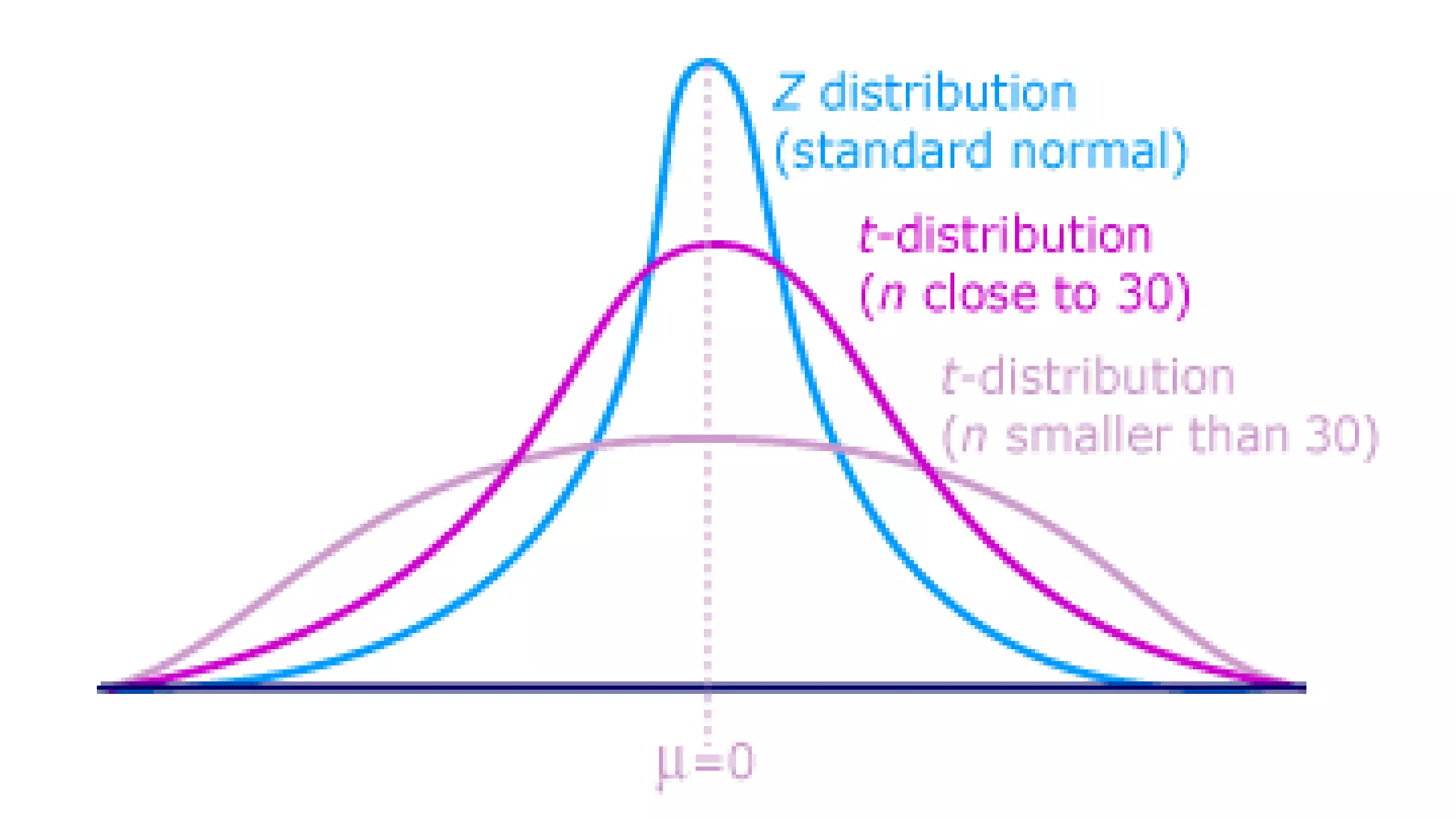


- The sample mean is the best estimate of the population mean and can be used to construct confidence intervals to estimate the true population mean. - There are two situations when estimating a population mean: when the population standard deviation (σ) is known, and when σ is unknown. - When σ is known, a z-test is used. When σ is unknown, a t-test is used since the sample standard deviation is used to estimate the population standard deviation.


![ict_presentation_final_final_final[1].pptx](https://cdn.slidesharecdn.com/ss_thumbnails/ictpresentationfinalfinalfinal1-251230145259-2b4839bd-thumbnail.jpg?width=640&height=640&fit=bounds)


