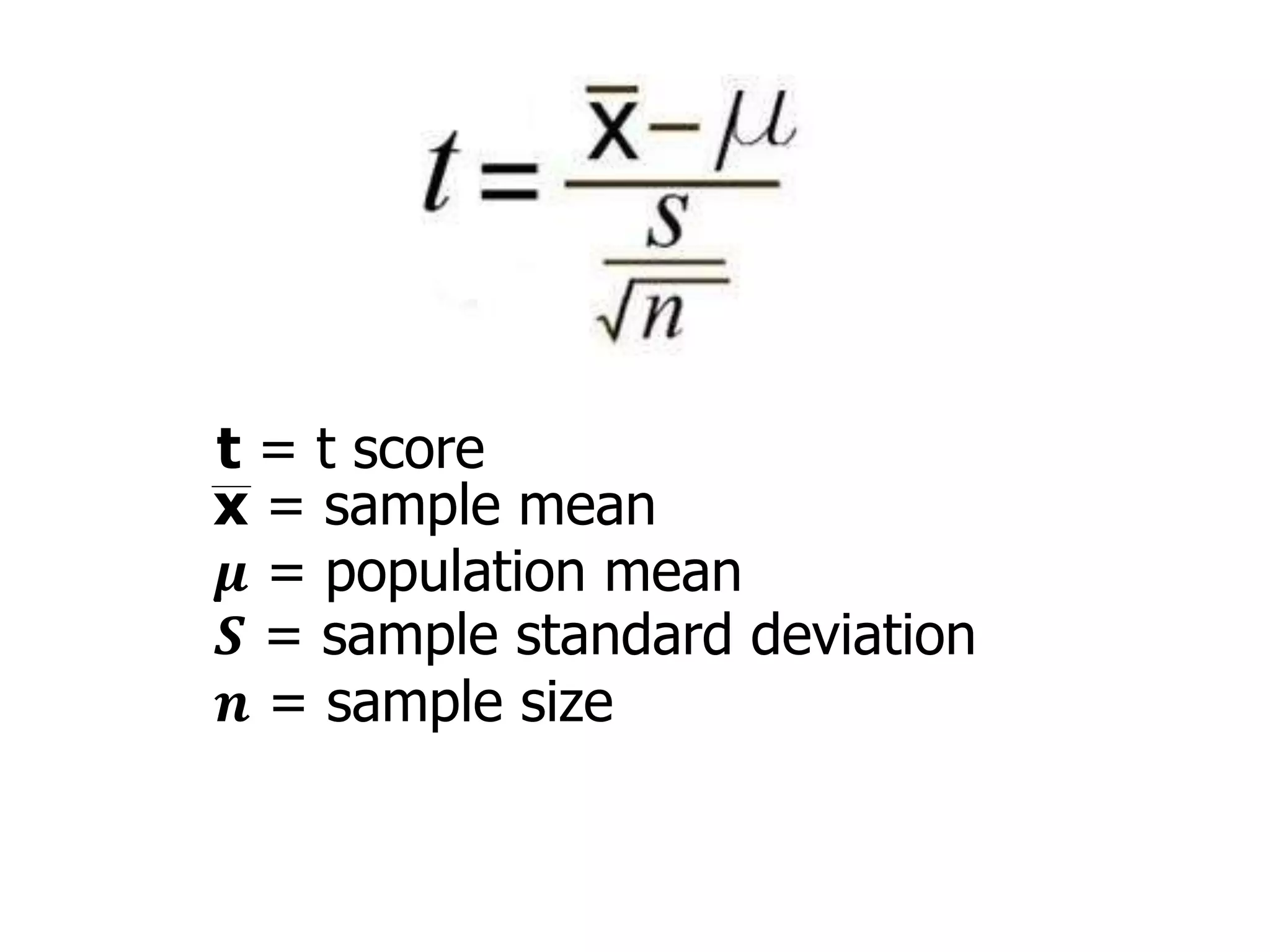
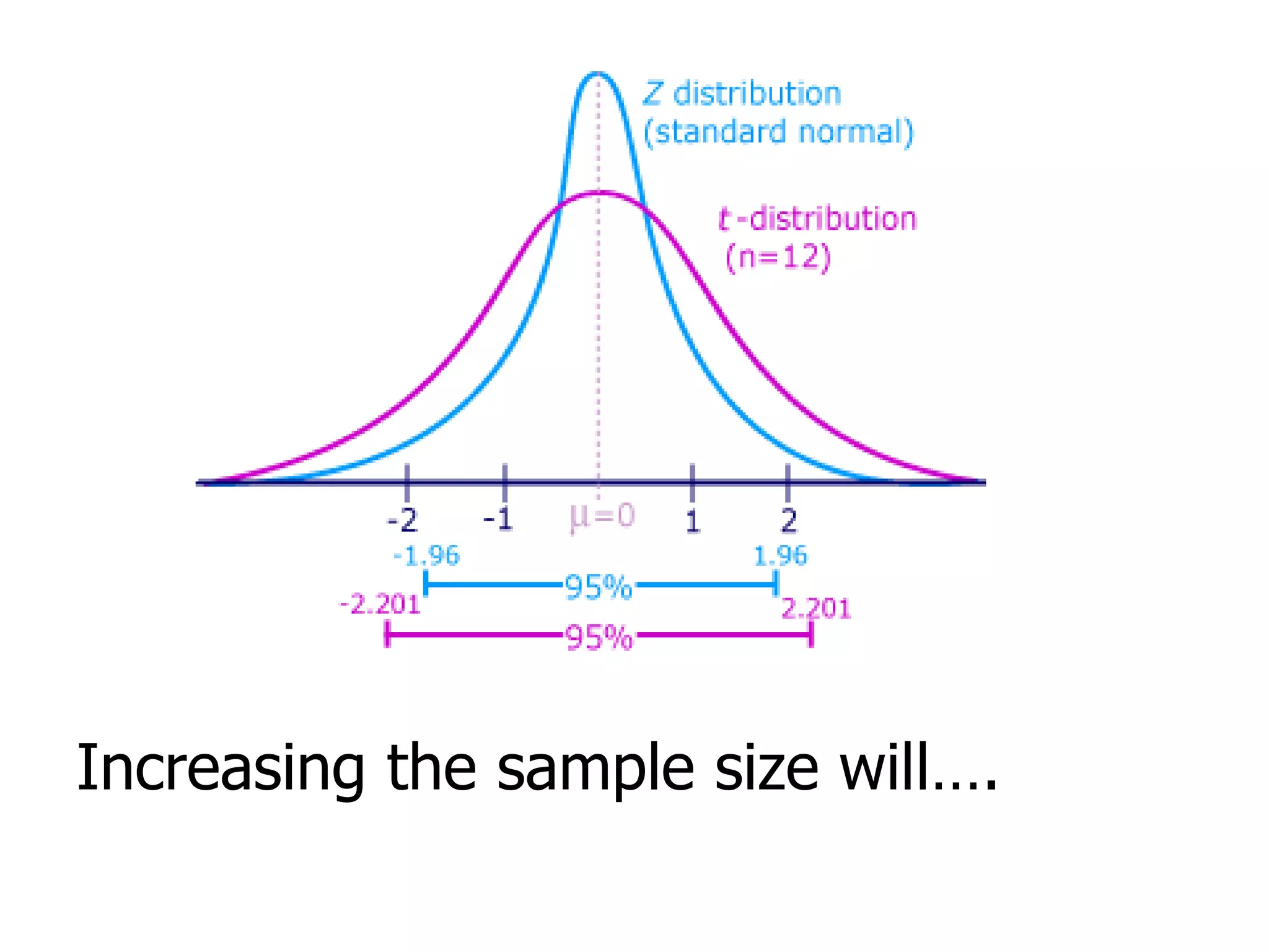
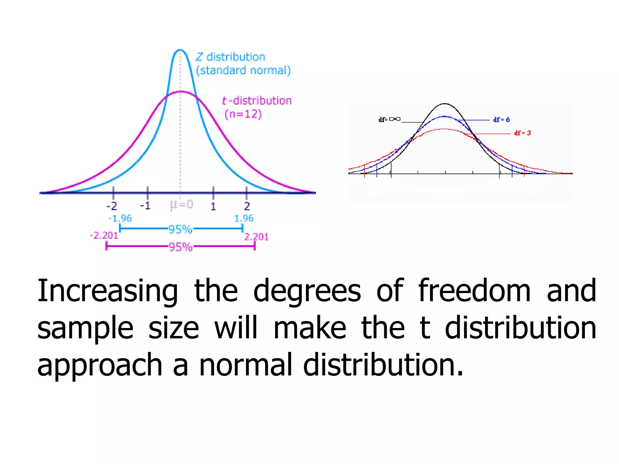
t distribution
(Student’s t distribution)
In the previous discussions, it
was shown that when the
population is normally distributed,
or when the sample size is large
enough, the sampling distribution of
the mean is normally distributed.
And of course, the bell curve is very
handy to use.
However, in many cases
where we can only obtain small
sizes, the normal distribution
does not hold true. Instead, we
use the t distribution which is
the distribution of t-scores.
t = t score
x = sample mean
𝝁 = population mean
𝑺 = sample standard deviation
𝒏 = sample size
EXAMPLE 1
Find the t-score for a sample
size of 16 taken from a population
with mean 10 when the sample
mean is 12 and the sample
standard deviation is 1.5.
Degrees of freedom
- the number of observations in
a data set that are free to change
without changing the mean.
For a single group test
𝑑𝑓 = 𝑁 − 1
For 2-group tests
𝑑𝑓 = 𝑁1 + 𝑁2 − 2
PROPERTIES of a t distribution
1. The distribution has mean 0.
2. The distribution is symmetric
about the mean.
3. The variance is equal to
𝑑𝑓
𝑑𝑓−2
.
4. The variance is always greater
than 1, but approaches 1 when
df gets bigger.
What if n approaches infinity?
The t distribution also
approaches the standard normal
distribution.
Increasing the sample size will….
Increasing the degrees of freedom will…
Increasing the degrees of freedom and
sample size will make the t distribution
approach a normal distribution.
The critical value is the thin line
between rejection and acceptance.
The confidence
interval is actually
the acceptance
region.
The t TABLE
1. The critical region appears at
the top.
2. The degrees of freedom are on
the leftmost section.
3. Confidence interval are at the
bottom.
EXAMPLE 2
Find the t-score below which
we can expect 99% of sample
means will fall if samples of size 16
are taken from a normally
distributed population.
EXAMPLE 2
SOLUTION
1 − 𝛼 = 0.99
𝛼 = 0.01
𝑑𝑓 = 𝑛 − 1
𝑡0.99 = −𝑡0.01
𝑑𝑓 = 15
𝑡0.99 = −𝑡0.01 = −2.602
EXAMPLE 3
If a random sample of size 25
drawn from a normal population
gives a mean of 60 and a standard
deviation of 4, find the range of t-
scores where we can expect to find
the middle 95% of all sample
means.
EXAMPLE 4
Compute the probability that
𝑃 (−𝑡0.05 < 𝑡 < 𝑡0.10).

T distribution

  • 1.
  • 3.
    In the previousdiscussions, it was shown that when the population is normally distributed, or when the sample size is large enough, the sampling distribution of the mean is normally distributed. And of course, the bell curve is very handy to use.
  • 4.
    However, in manycases where we can only obtain small sizes, the normal distribution does not hold true. Instead, we use the t distribution which is the distribution of t-scores.
  • 5.
    t = tscore x = sample mean 𝝁 = population mean 𝑺 = sample standard deviation 𝒏 = sample size
  • 6.
    EXAMPLE 1 Find thet-score for a sample size of 16 taken from a population with mean 10 when the sample mean is 12 and the sample standard deviation is 1.5.
  • 7.
    Degrees of freedom -the number of observations in a data set that are free to change without changing the mean. For a single group test 𝑑𝑓 = 𝑁 − 1 For 2-group tests 𝑑𝑓 = 𝑁1 + 𝑁2 − 2
  • 8.
    PROPERTIES of at distribution 1. The distribution has mean 0. 2. The distribution is symmetric about the mean. 3. The variance is equal to 𝑑𝑓 𝑑𝑓−2 . 4. The variance is always greater than 1, but approaches 1 when df gets bigger.
  • 9.
    What if napproaches infinity? The t distribution also approaches the standard normal distribution.
  • 10.
    Increasing the samplesize will….
  • 11.
    Increasing the degreesof freedom will…
  • 12.
    Increasing the degreesof freedom and sample size will make the t distribution approach a normal distribution.
  • 13.
    The critical valueis the thin line between rejection and acceptance.
  • 14.
    The confidence interval isactually the acceptance region.
  • 15.
    The t TABLE 1.The critical region appears at the top. 2. The degrees of freedom are on the leftmost section. 3. Confidence interval are at the bottom.
  • 16.
    EXAMPLE 2 Find thet-score below which we can expect 99% of sample means will fall if samples of size 16 are taken from a normally distributed population.
  • 17.
    EXAMPLE 2 SOLUTION 1 −𝛼 = 0.99 𝛼 = 0.01 𝑑𝑓 = 𝑛 − 1 𝑡0.99 = −𝑡0.01 𝑑𝑓 = 15 𝑡0.99 = −𝑡0.01 = −2.602
  • 18.
    EXAMPLE 3 If arandom sample of size 25 drawn from a normal population gives a mean of 60 and a standard deviation of 4, find the range of t- scores where we can expect to find the middle 95% of all sample means.
  • 19.
    EXAMPLE 4 Compute theprobability that 𝑃 (−𝑡0.05 < 𝑡 < 𝑡0.10).