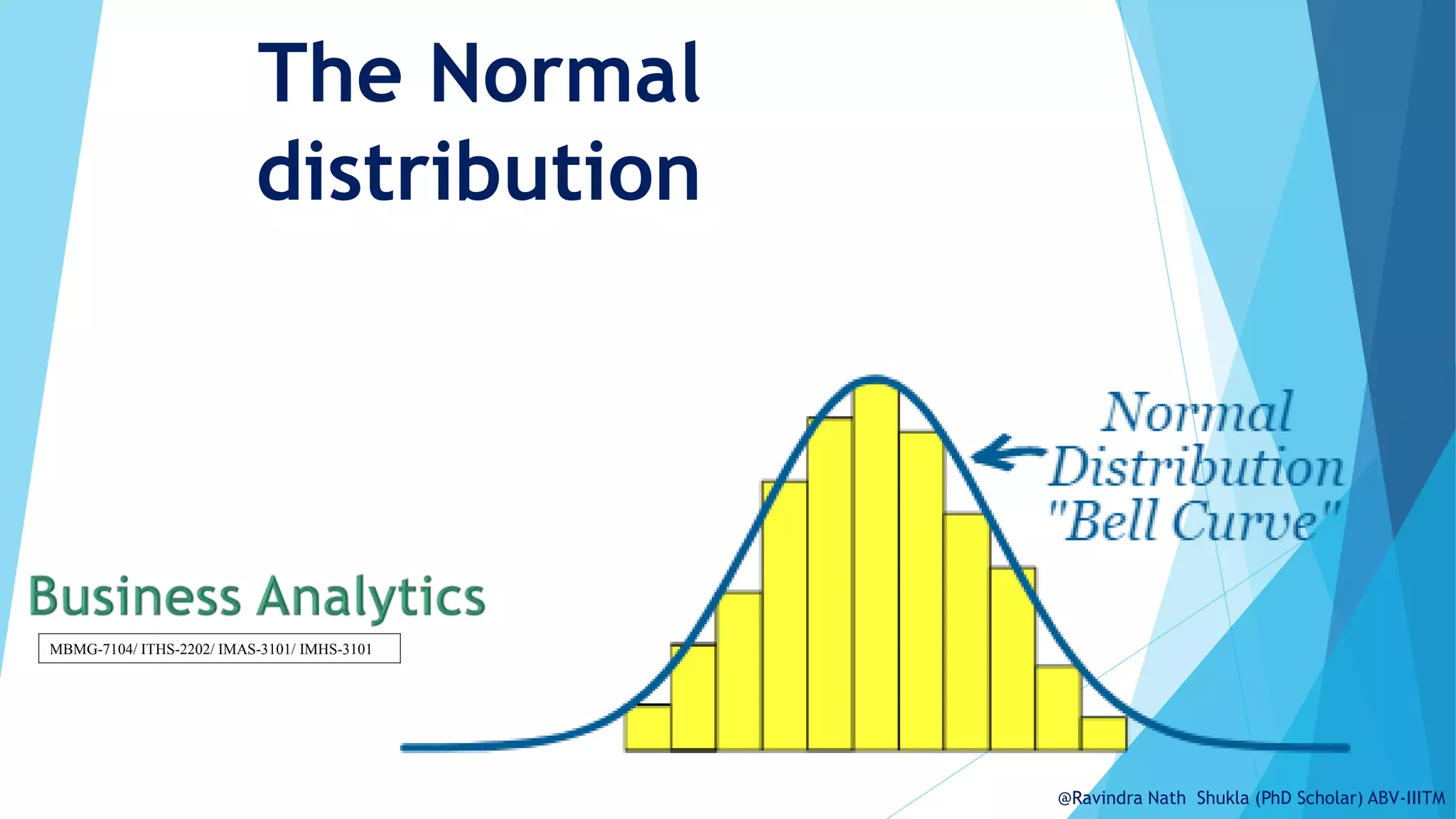
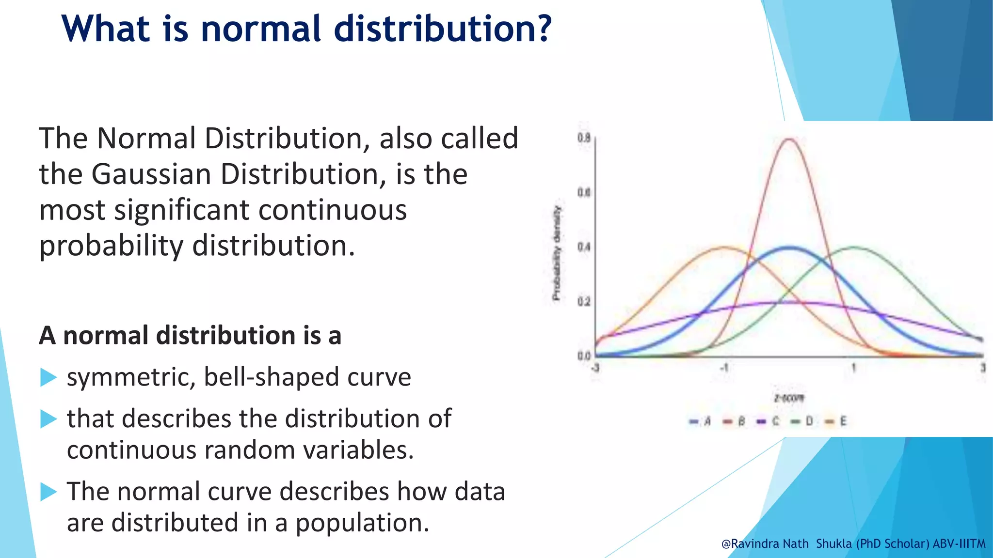
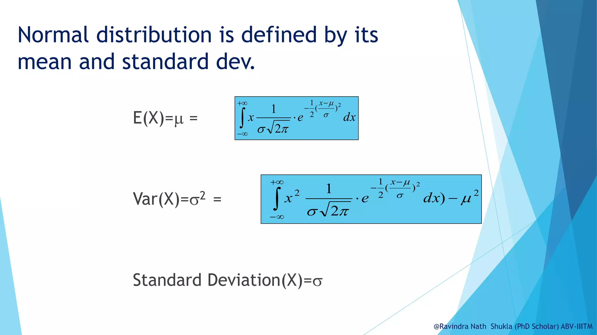
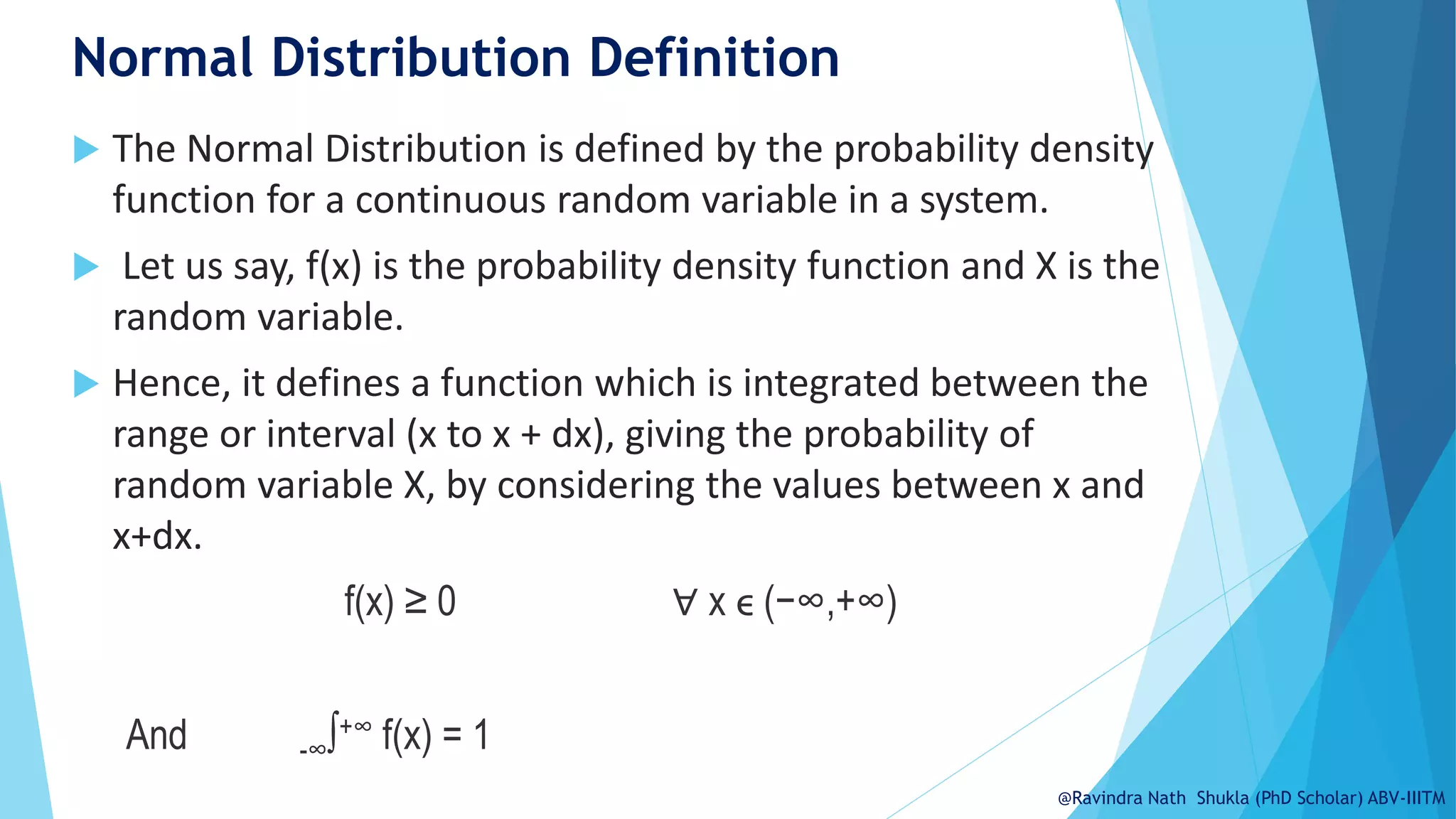
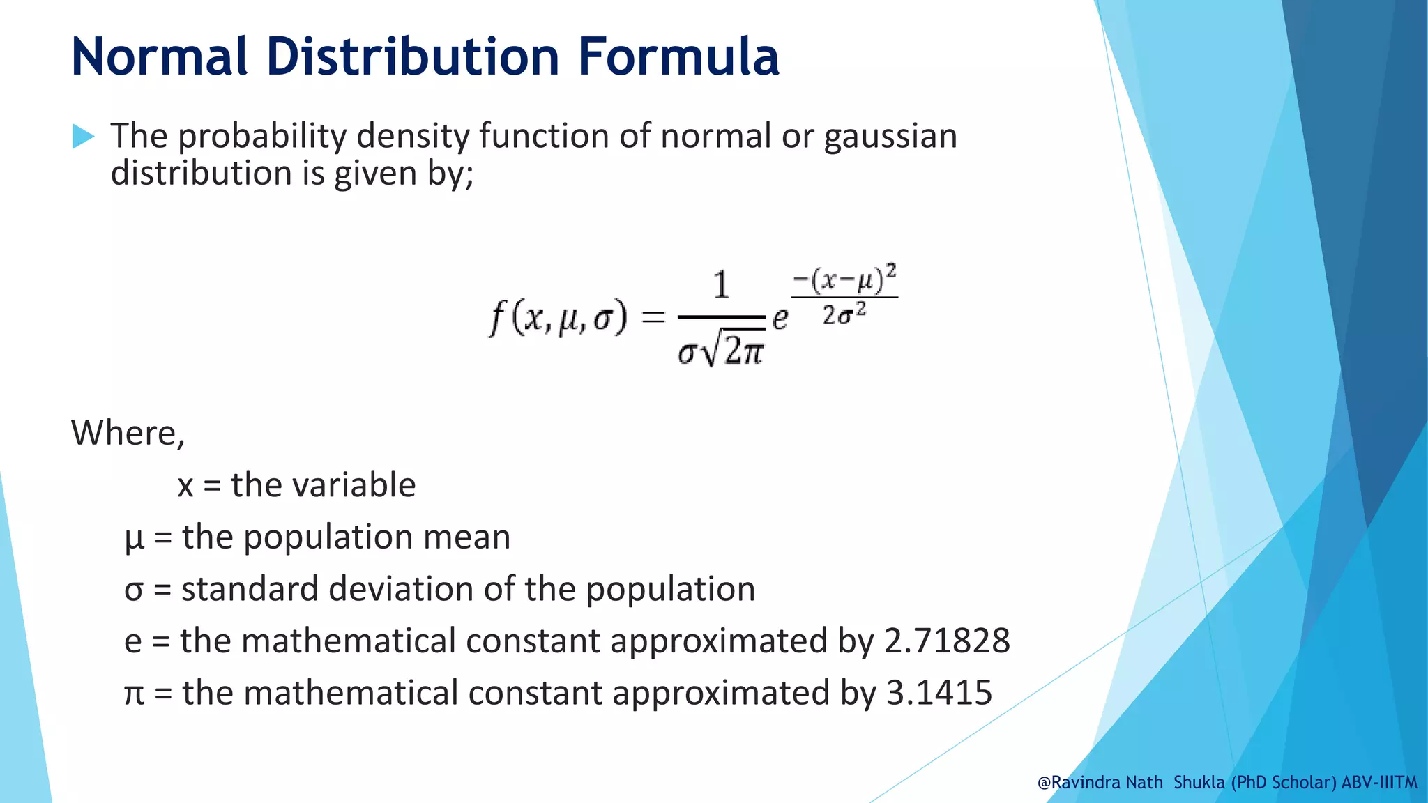
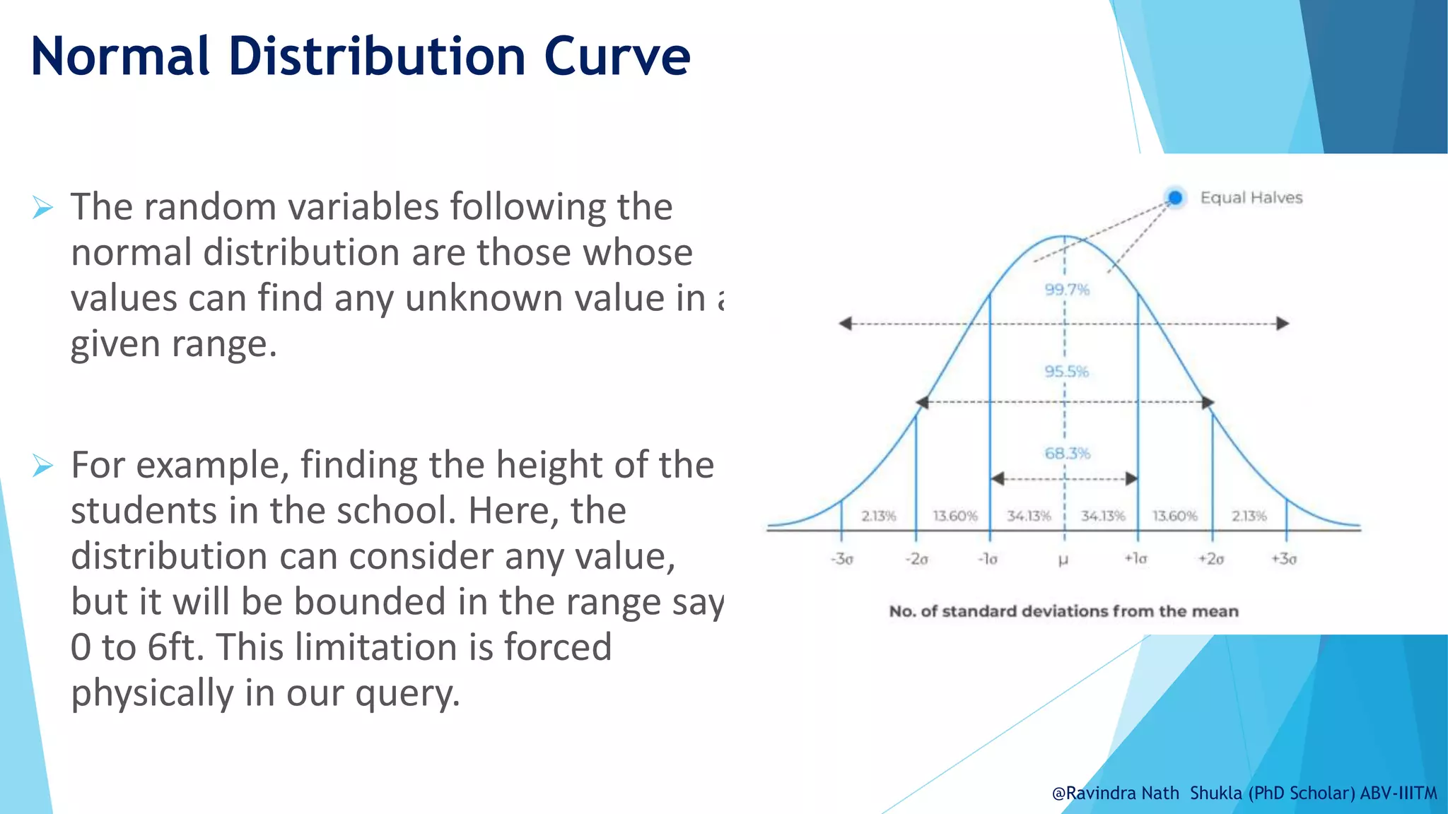
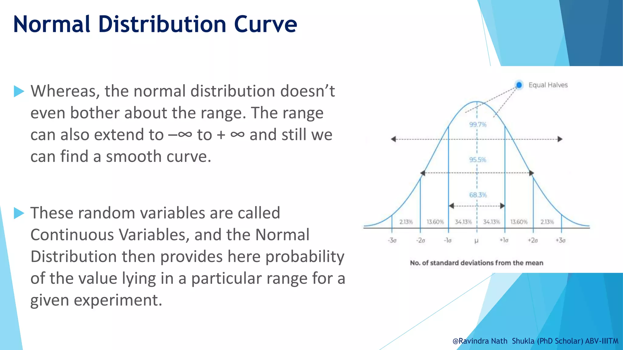
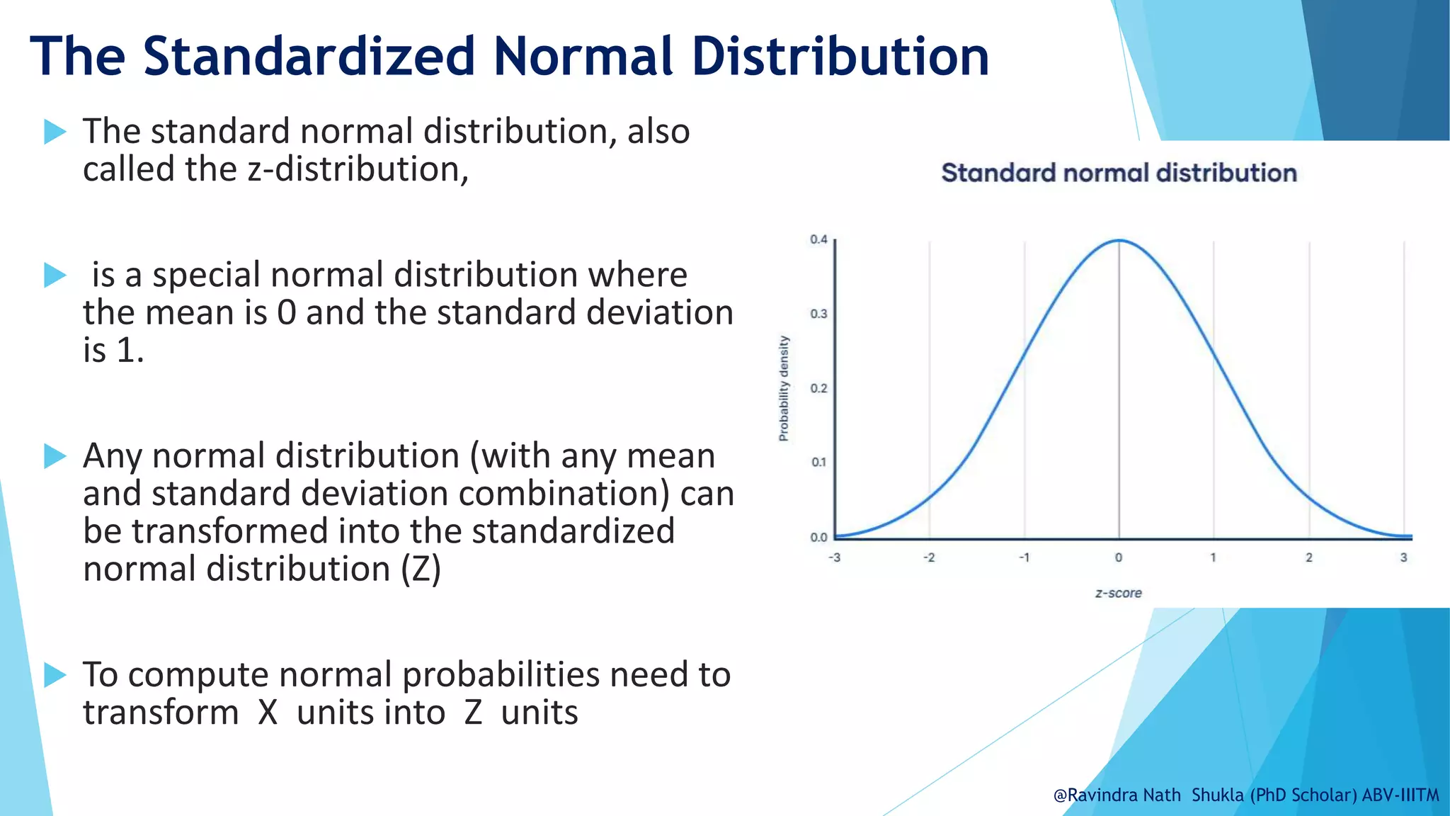
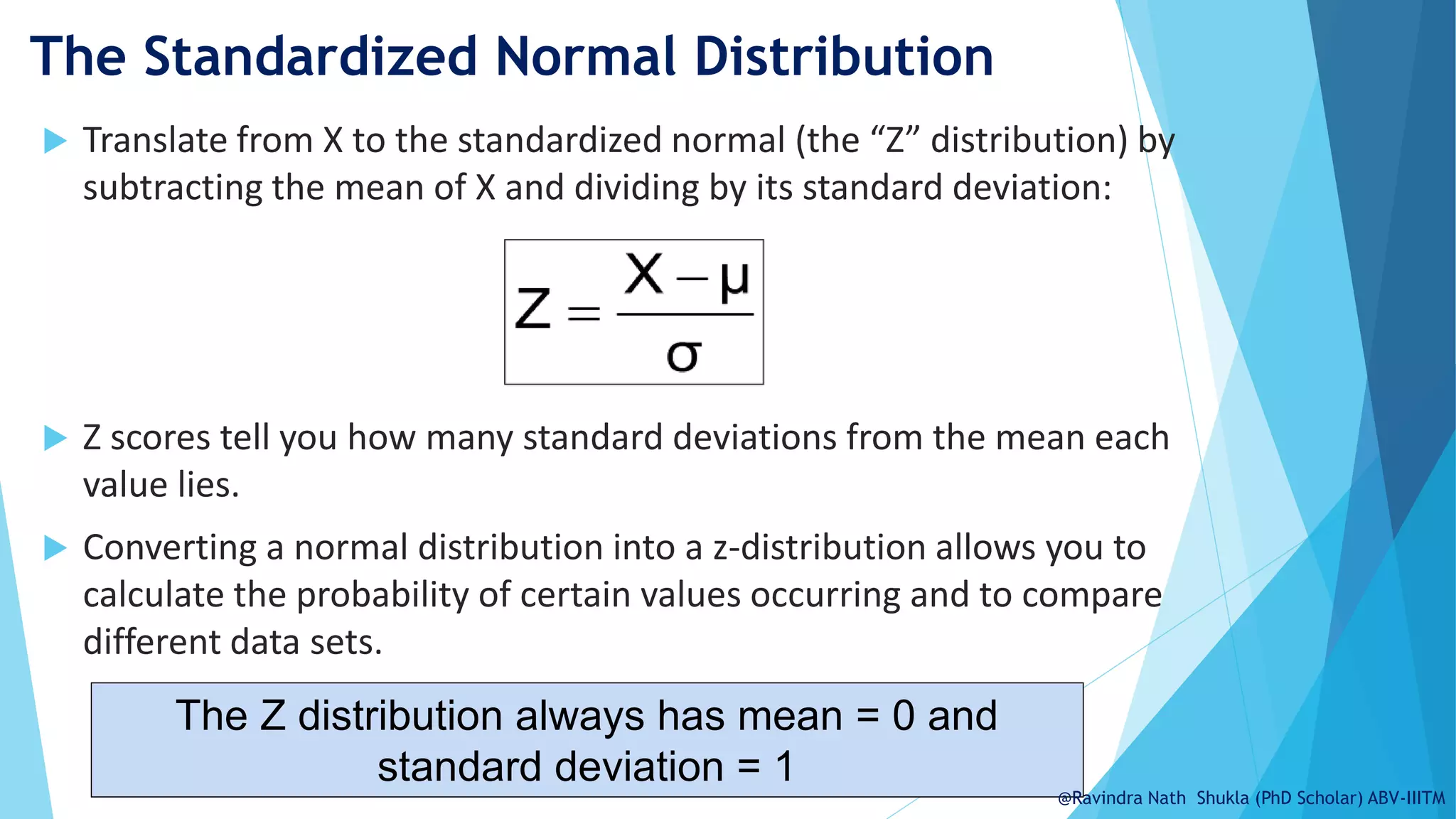
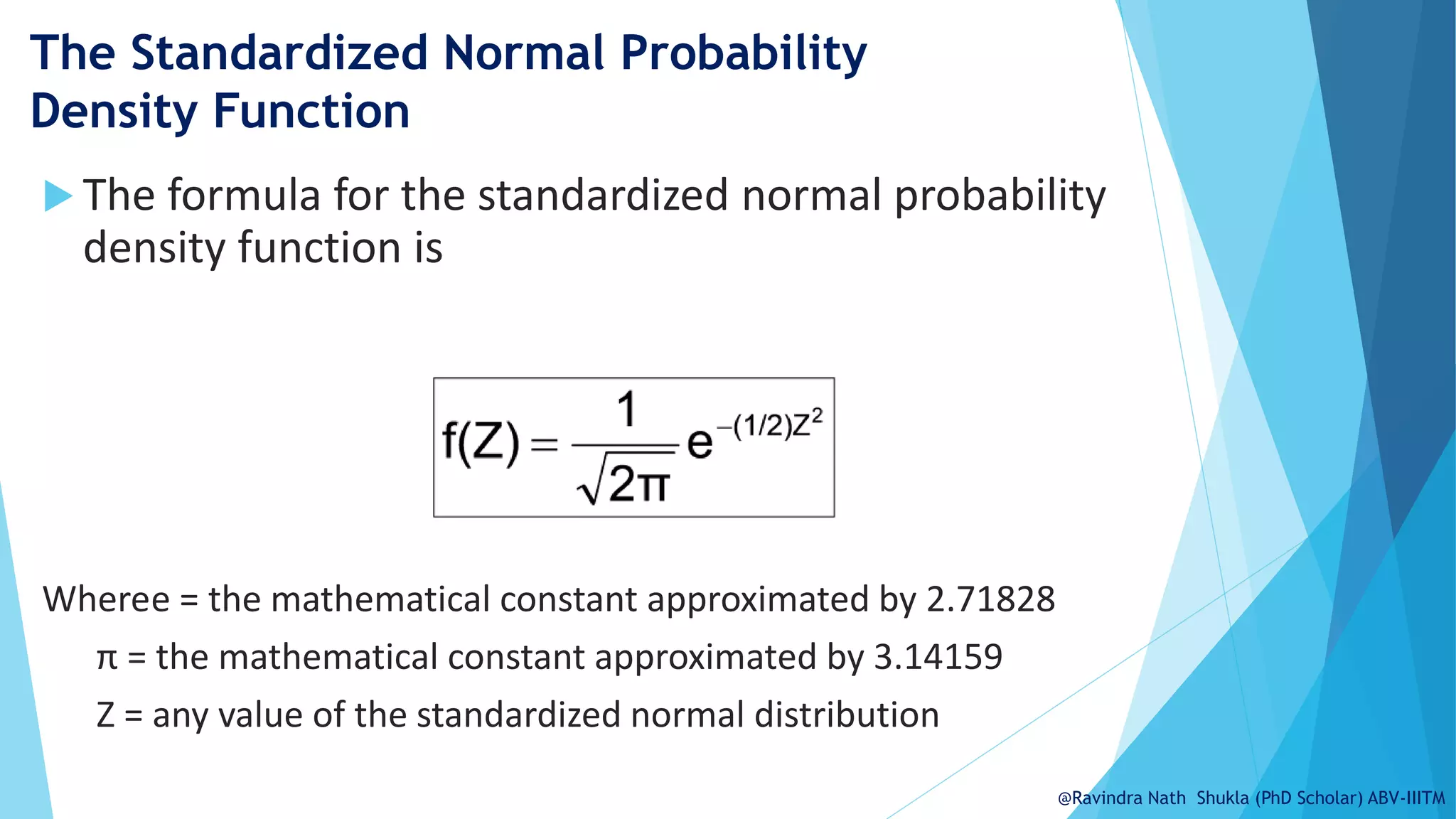
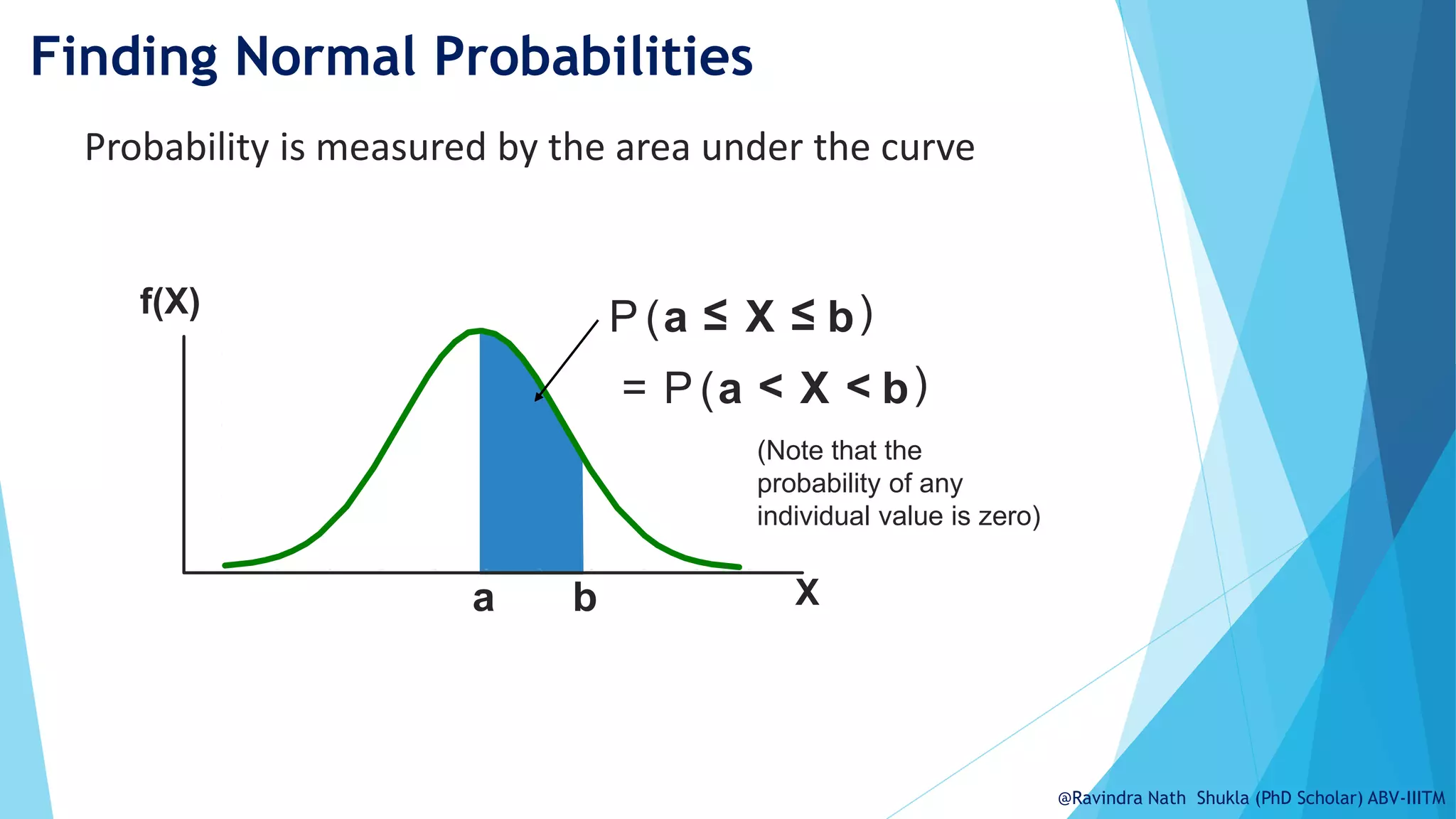
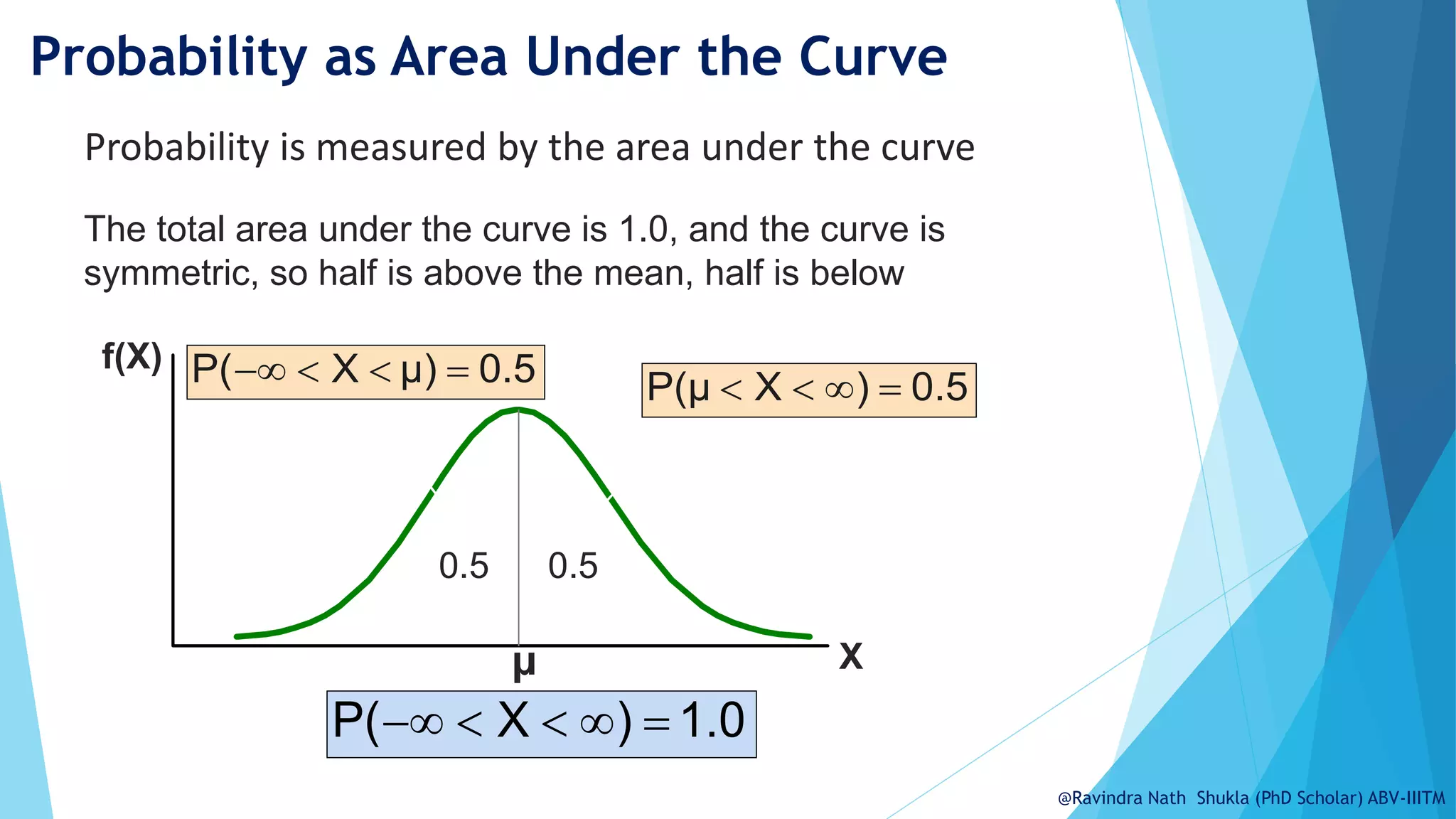
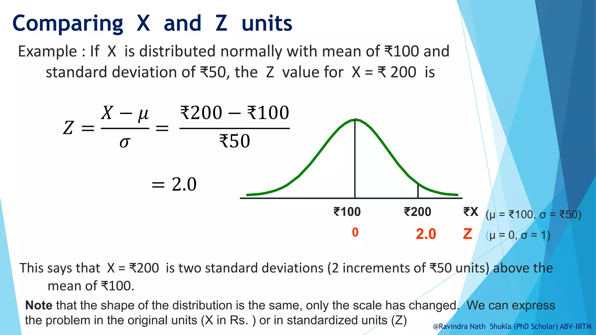
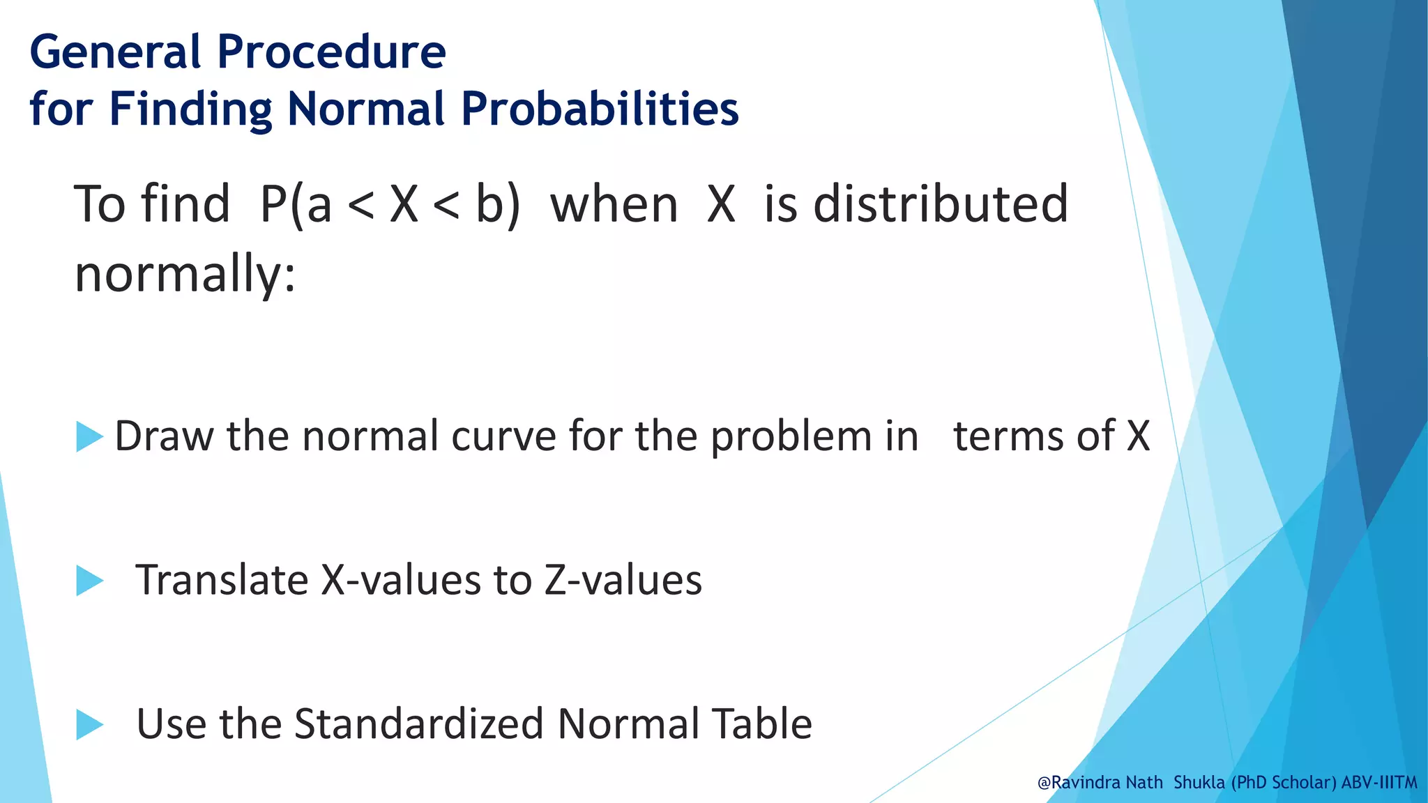
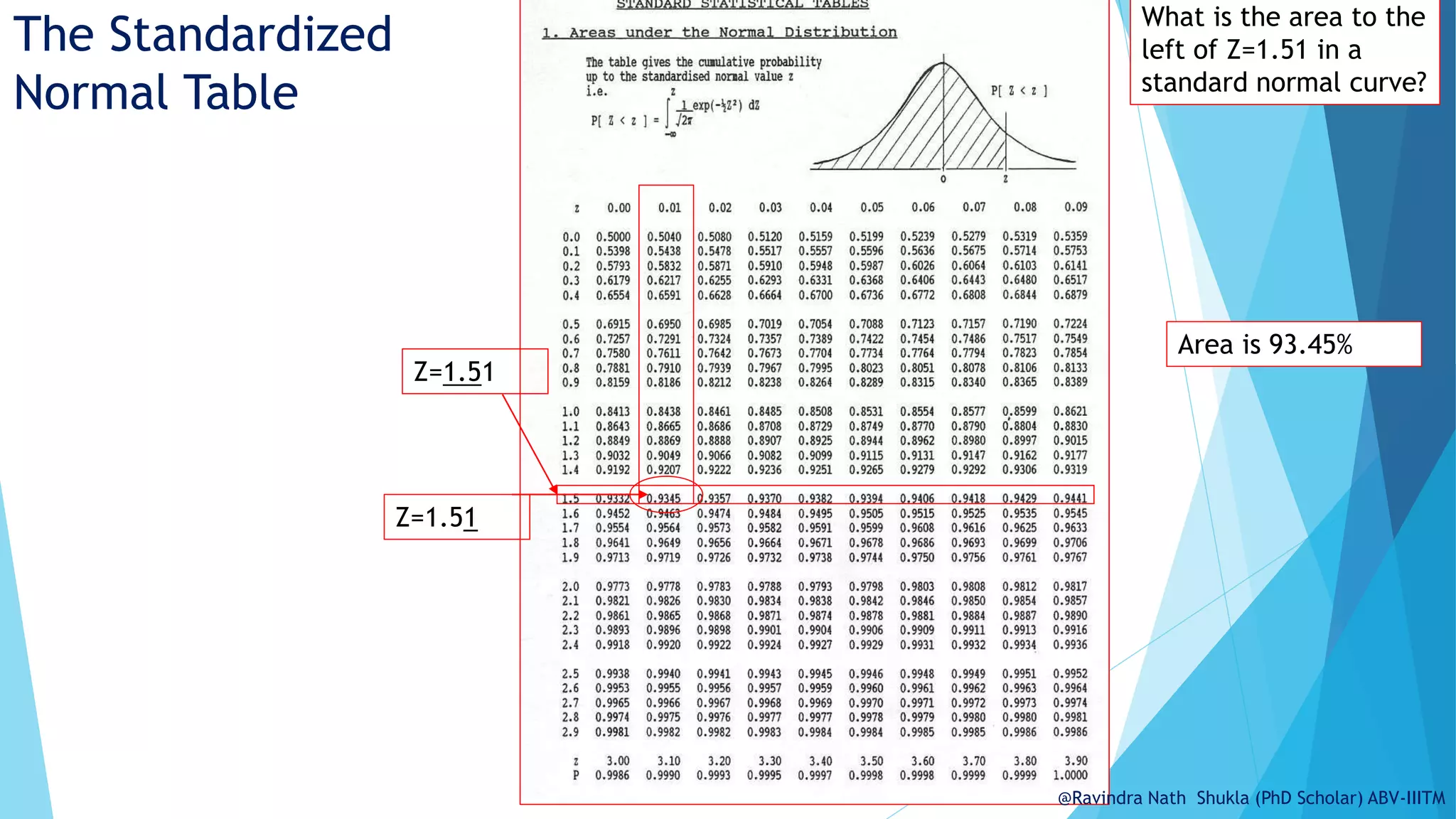
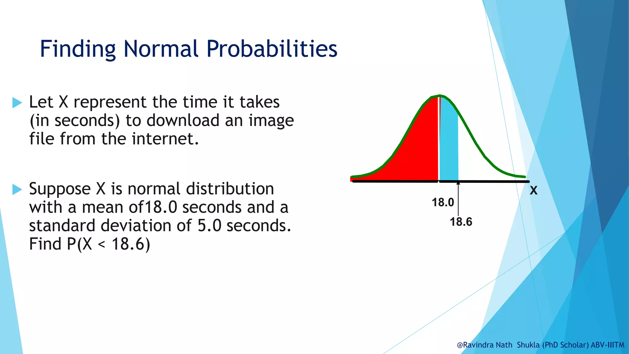
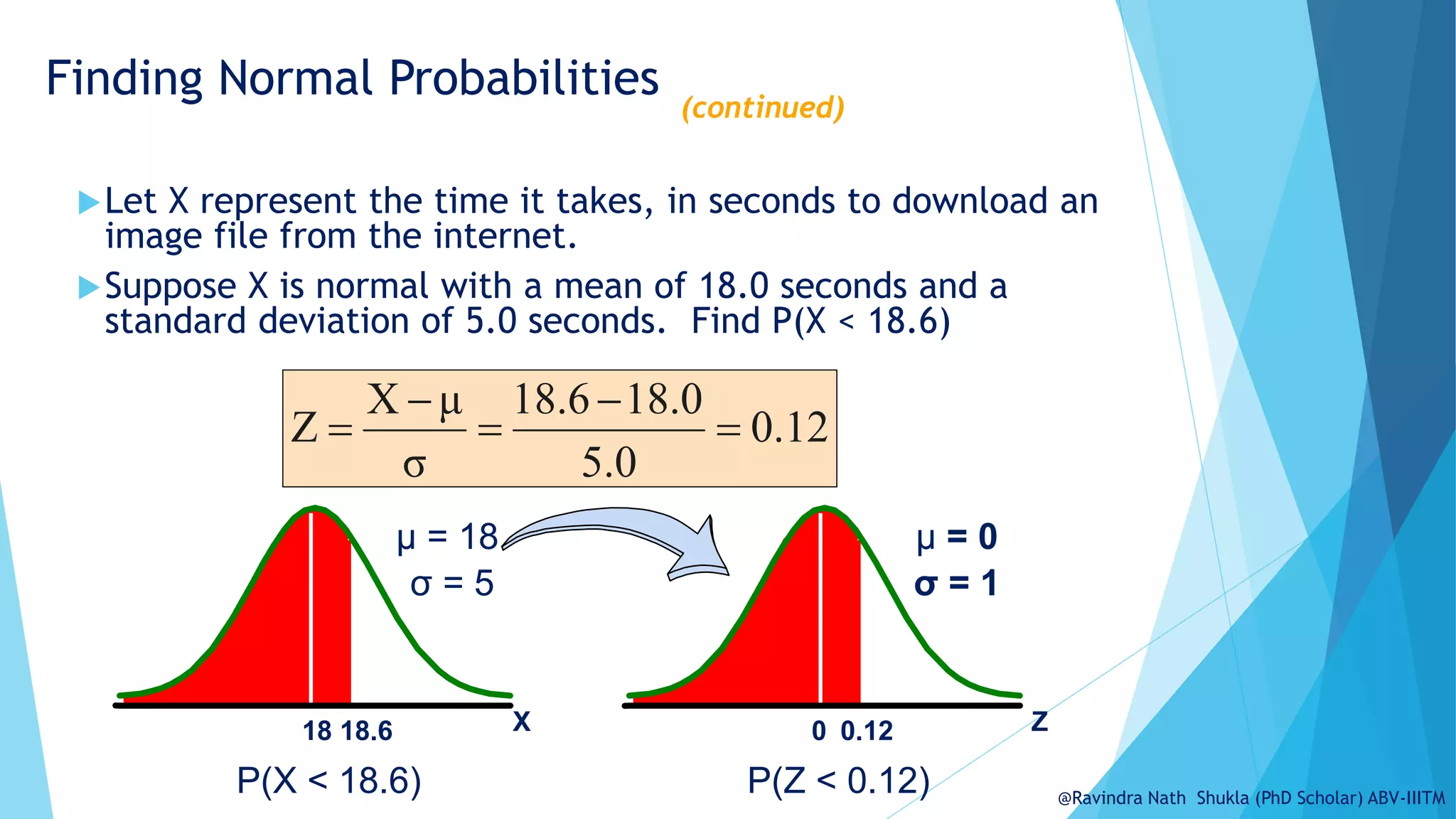
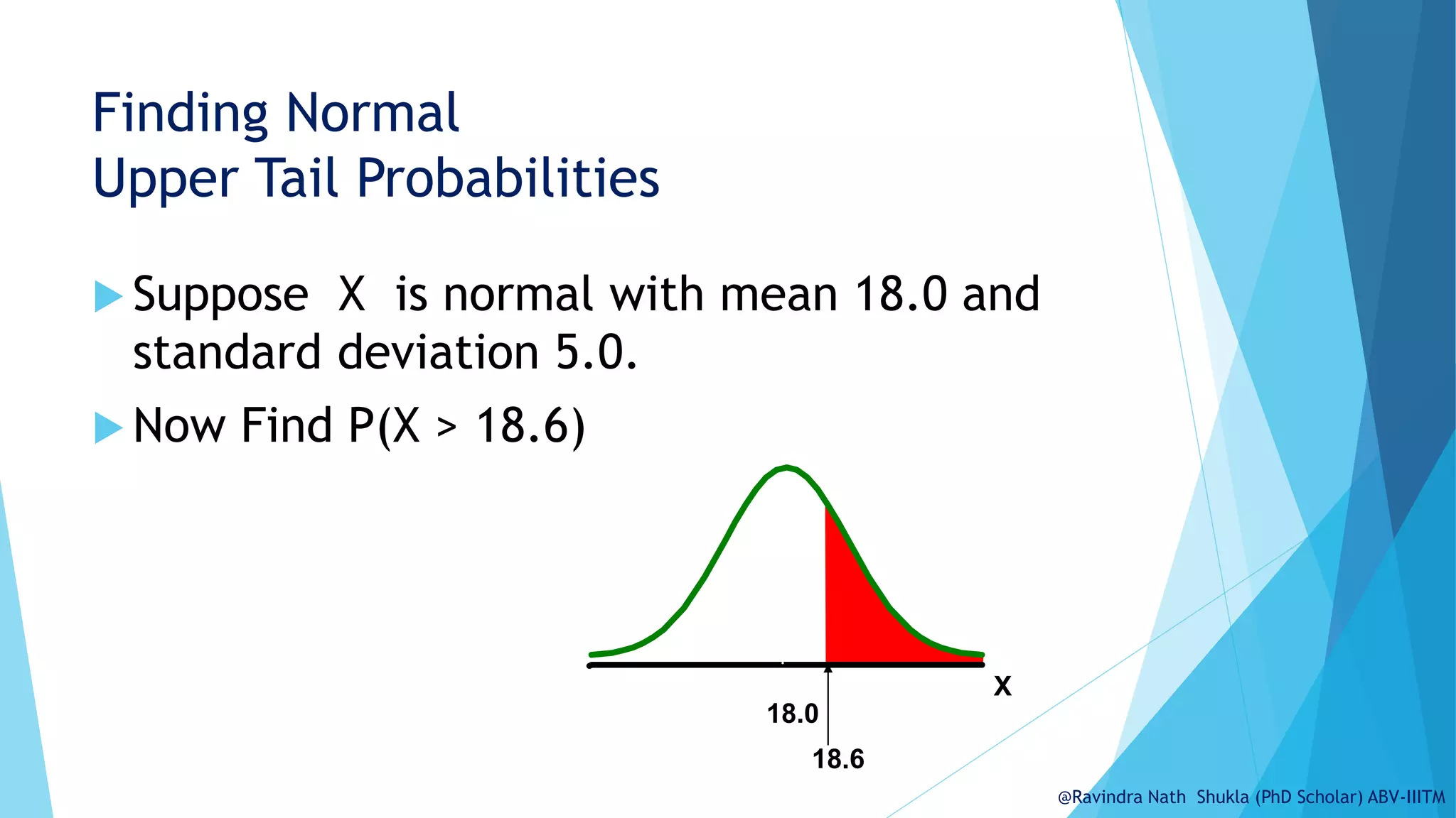
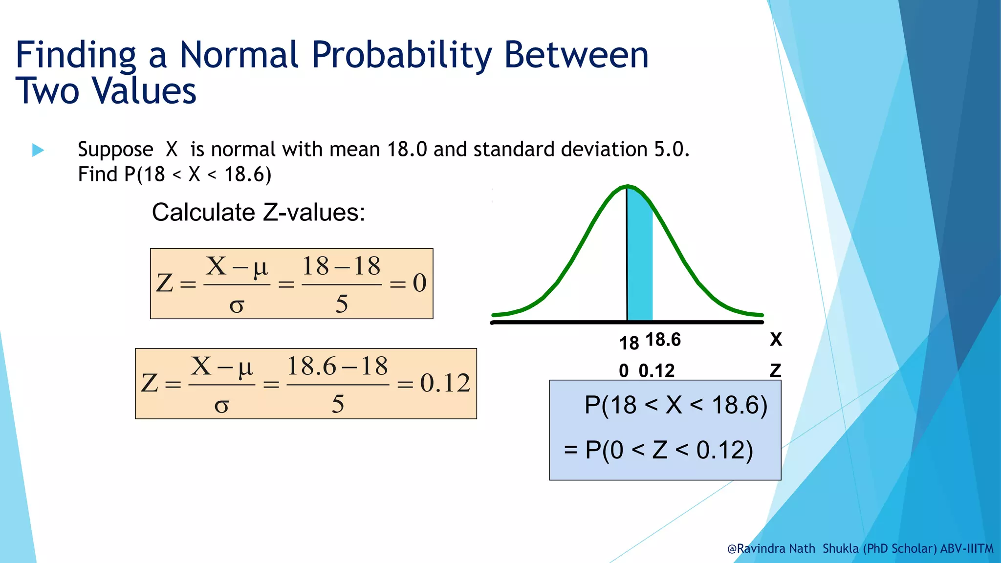
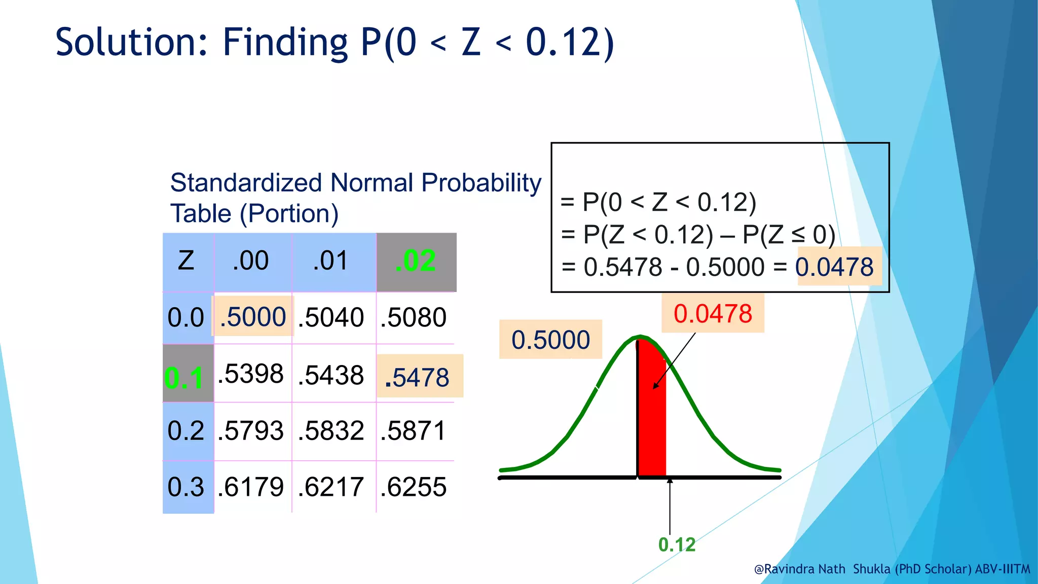
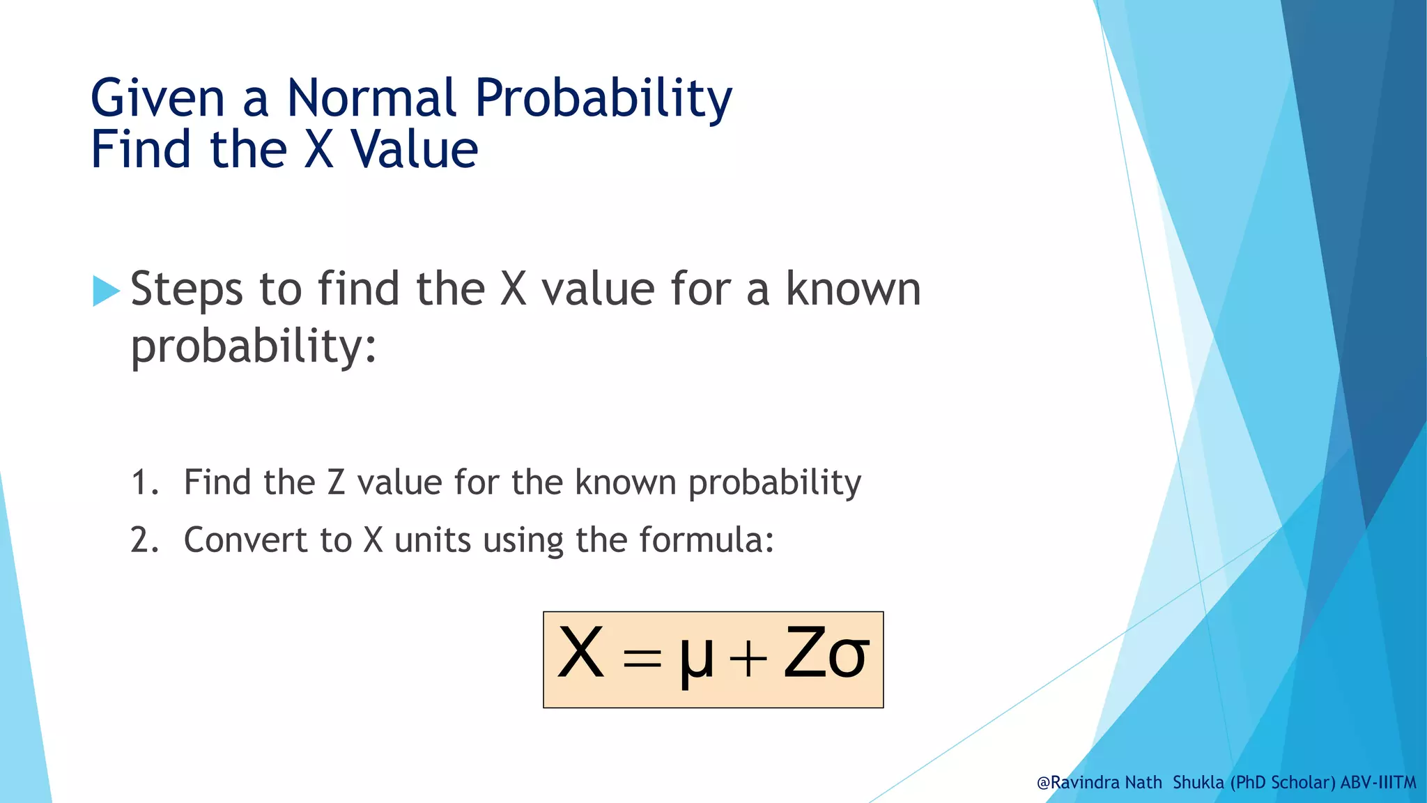
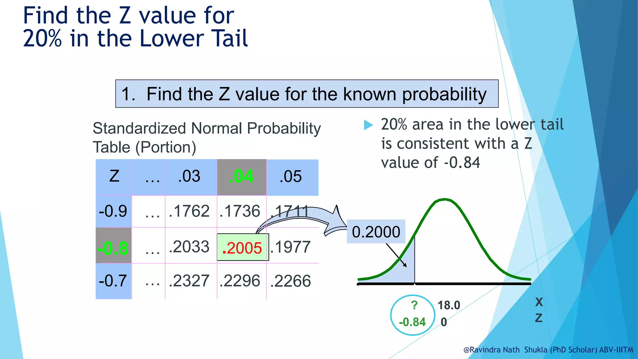
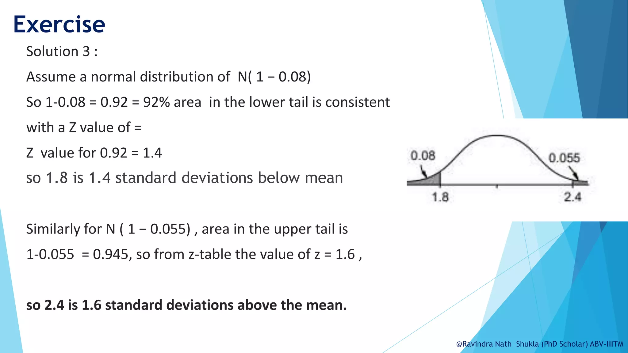
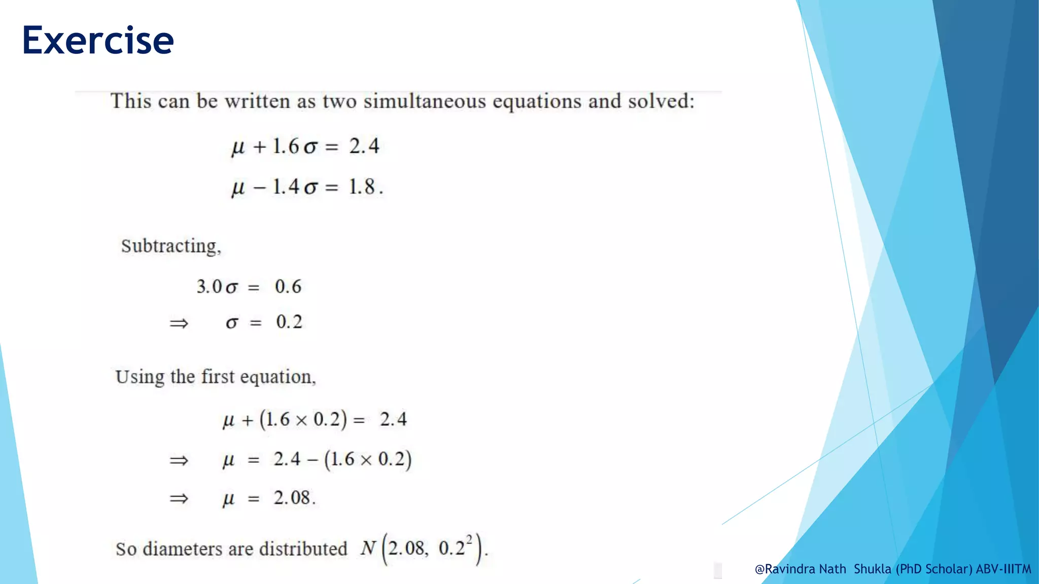
This ppt is a part of Business Analytics course.
Normal distribution : -
The Normal Distribution, also called the Gaussian Distribution, is the most significant continuous probability distribution.
A normal distribution is a
symmetric, bell-shaped curve
that describes the distribution of continuous random variables.
The normal curve describes how data are distributed in a population.
A large number of random variables are either nearly or exactly represented by the normal distribution
The normal distribution can be used to represent a wide range of data, such as test scores, height measurements, and weights of people in a population.
BMI (kg/m2)
22.1
23.4
24.8
26.2
27.6
28.9
30.3
31.6
32.9
34.2
35.5
36.8
38.1
39.4
The sample mean is 29.1 kg/m2 and the sample standard
deviation is 4.2 kg/m2. Test the hypothesis that the
population mean BMI is 30 kg/m2 at 5% level of
significance.
The document discusses the standard normal distribution and provides examples of how to calculate probabilities for a normal distribution. It defines the standard normal distribution as having a mean of 0 and standard deviation of 1. It then shows how to standardize a normal variable by subtracting the mean and dividing by the standard deviation. Examples calculate probabilities such as the area under or above a value and between two values by using the standard normal distribution table.
Hypothesis Test _One-sample t-test, Z-test, Proportion Z-testRavindra Nath Shukla
This document discusses hypothesis testing concepts including the null and alternative hypotheses, type I and II errors, and the hypothesis testing process. It provides examples of hypothesis testing for a mean where the population standard deviation is known (z-test) and unknown (t-test). The document outlines the 6 steps in hypothesis testing and provides examples using both the critical value approach and p-value approach. It discusses the relationship between hypothesis testing and confidence intervals.
Normal Distribution
Properties of Normal Distribution
Empirical rule of normal distribution
Normality limits
Standard normal distribution(z-score/ SND)
Properties of SND
Use of z/normal table
Solved examples
Probability ,Binomial distribution, Normal distribution, Poisson’s distributi...AZCPh
Definition of probability, Binomial distribution, Normal distribution Poisson’s distribution, properties – problems .
Mathematical / classical probability equation , The multiplicative law of probability when are not mutually exclusive, THE BINOMIAL DISTRIBUTION – with continuous data, The standard normal probability curve
The document discusses various statistical concepts including range, mean deviation, variance, and standard deviation. It provides formulas and steps to calculate each measure. The range is the distance between the highest and lowest values. Mean deviation measures the average deviation from the mean. Variance is the average of the squared deviations from the mean and standard deviation is the square root of the variance, representing the average distance from the mean. Examples are given to demonstrate calculating each measure for both ungrouped and grouped data.
Hypothesis testing involves proposing and testing hypotheses, or predictions, about relationships between variables. There are four main types of hypotheses: null, alternative, directional, and non-directional. The null hypothesis proposes no relationship between variables, while the alternative hypothesis contradicts the null. Directional hypotheses predict the nature of a relationship, while non-directional hypotheses do not. Common statistical tests used for hypothesis testing include the z-test, t-test, chi-square test, and F-test. Hypothesis testing is a crucial part of the scientific method for assessing theories through empirical observation.
This document discusses confidence intervals, which provide a range of values that is likely to include an unknown population parameter based on a sample statistic. It defines key concepts like confidence level, confidence limits, and factors that determine how to set the confidence interval like sample size, population variability, and precision of values. It explains how larger sample sizes and more precise measurements result in narrower confidence intervals. Applications to clinical trials are discussed, showing how sample size impacts the ability to make definitive recommendations based on trial results.
Regression analysis is a statistical technique used to estimate the relationships between variables. It allows one to predict the value of a dependent variable based on the value of one or more independent variables. The document discusses simple linear regression, where there is one independent variable, as well as multiple linear regression which involves two or more independent variables. Examples of linear relationships that can be modeled using regression analysis include price vs. quantity, sales vs. advertising, and crop yield vs. fertilizer usage. The key methods for performing regression analysis covered in the document are least squares regression and regressions based on deviations from the mean.
Regression analysis is a statistical technique for predicting a dependent variable based on one or more independent variables. Simple linear regression fits a straight line to the data to predict a continuous dependent variable (y) from a single independent variable (x). The output is an equation of the form y= b0 + b1x + ε, where b0 is the y-intercept, b1 is the slope, and ε is the error. Multiple linear regression extends this to include more than one independent variable. Regression analysis calculates the "best fit" line that minimizes the residuals, or differences between predicted and observed y values.
The central limit theorem states that the sampling distribution of the sample mean approaches a normal distribution as the sample size increases, even if the population is not normally distributed. It provides the mean and standard deviation of the sampling distribution of the sample mean. The document gives the definition of the central limit theorem and provides an example of how to use it to calculate probabilities related to the sample mean of a large normally distributed population.
The document provides an overview of hypothesis testing. It begins by defining a hypothesis test and its purpose of ruling out chance as an explanation for research study results. It then outlines the logic and steps of a hypothesis test: 1) stating hypotheses, 2) setting decision criteria, 3) collecting data, 4) making a decision. Key concepts discussed include type I and type II errors, statistical significance, test statistics like the z-score, and assumptions of hypothesis testing. Factors that can influence a hypothesis test like effect size, sample size, and alpha level are also covered.
The document discusses the normal distribution, which produces a symmetrical bell-shaped curve. It has two key parameters - the mean and standard deviation. According to the empirical rule, about 68% of values in a normal distribution fall within one standard deviation of the mean, 95% within two standard deviations, and 99.7% within three standard deviations. The normal distribution is commonly used to model naturally occurring phenomena that tend to cluster around an average value, such as heights or test scores.
Multiple regression analysis allows researchers to examine the relationship between one dependent or outcome variable and two or more independent or predictor variables. It extends simple linear regression to model more complex relationships. Stepwise regression is a technique that automates the process of building regression models by sequentially adding or removing variables based on statistical criteria. It begins with no variables in the model and adds variables one at a time based on their contribution to the model until none improve it significantly.
This document provides an introduction to probability theory and different probability distributions. It begins with defining probability as a quantitative measure of the likelihood of events occurring. It then covers fundamental probability concepts like mutually exclusive events, additive and multiplicative laws of probability, and independent events. The document also introduces random variables and common probability distributions like the binomial, Poisson, and normal distributions. It provides examples of how each distribution is used and concludes with characteristics of the normal distribution.
The document discusses the Chi-square (χ2) test, which is a non-parametric test used to test hypotheses about distributions of frequencies across categories of data. It can be used to test for comparing variance and to test for independence between two variables. The summary provides steps for applying the Chi-square test, including calculating expected frequencies, observed vs expected values, the Chi-square statistic, and comparing it to critical values. An example application to test the effectiveness of vaccination in preventing smallpox is shown.
Through this ppt you could learn what is Wilcoxon Signed Ranked Test. This will teach you the condition and criteria where it can be run and the way to use the test.
The document discusses the standard normal distribution. It defines the standard normal distribution as having a mean of 0, a standard deviation of 1, and a bell-shaped curve. It provides examples of how to find probabilities and z-scores using the standard normal distribution table or calculator. For example, it shows how to find the probability of an event being below or above a given z-score, or between two z-scores. It also shows how to find the z-score corresponding to a given cumulative probability.
This document provides an overview of non-parametric statistics. It defines non-parametric tests as those that make fewer assumptions than parametric tests, such as not assuming a normal distribution. The document compares and contrasts parametric and non-parametric tests. It then explains several common non-parametric tests - the Mann-Whitney U test, Wilcoxon signed-rank test, sign test, and Kruskal-Wallis test - and provides examples of how to perform and interpret each test.
The document discusses various statistical tests used for hypothesis testing, including parametric and non-parametric tests. Parametric tests like the z-test and t-test assume a normal distribution, while non-parametric tests like the chi-square test, sign test, and Mann-Whitney test make fewer assumptions. The z-test specifically compares a sample mean to a hypothesized population mean for large samples or when the population variance is known.
This presentation contains information about Mann Whitney U test, what is it, when to use it and how to use it. I have also put an example so that it may help you to easily understand it.
The document discusses parametric and non-parametric tests. It provides examples of commonly used non-parametric tests including the Mann-Whitney U test, Kruskal-Wallis test, and Wilcoxon signed-rank test. For each test, it gives the steps to perform the test and interpret the results. Non-parametric tests make fewer assumptions than parametric tests and can be used when the data is ordinal or does not meet the assumptions of parametric tests. They provide a distribution-free alternative for analyzing data.
Regression analysis is a statistical technique for modeling the relationship between variables. It can be used to predict the value of a dependent variable based on the value of one or more independent variables. The earliest and most common type of regression is linear regression, which finds the line of best fit to describe the relationship between two variables (e.g. y= a + bx). More advanced techniques allow for modeling nonlinear relationships and multiple independent variables. Regression analysis is widely used in fields like economics, sciences, and social sciences.
A research hypothesis is a statement created by researchers to speculate on the outcome of an experiment. Hypotheses are generated through inductive reasoning from observations and must be testable, falsifiable, and realistic. There are two types of errors in hypothesis testing: type I errors which incorrectly reject a true null hypothesis, and type II errors which fail to reject a false null hypothesis. Examples of hypotheses and errors are given for building inspections and the effects of fluoride in toothpaste.
The Normal Distribution:
There are different distributions namely Normal, Skewed, and Binomial etc.
Objectives:
Normal distribution its properties its use in biostatistics
Transformation to standard normal distribution
Calculation of probabilities from standard normal distribution using Z table.
Normal distribution:
- Certain data, when graphed as a histogram (data on the horizontal axis, frequency on the vertical axis), creates a bell-shaped curve known as a normal curve, or normal distribution.
- Two parameters define the normal distribution, the mean (µ) and the standard deviation (σ).
Properties of the Normal Distribution:
Normal distributions are symmetrical with a single central peak at the mean (average) of the data.
The shape of the curve is described as bell-shaped with the graph falling off evenly on either side of the mean.
Fifty percent of the distribution lies to the left of the mean and fifty percent lies to the right of the mean.
-The mean, the median, and the mode fall in the same place. In a normal distribution the mean = the median = the mode.
- The spread of a normal distribution is controlled by the
standard deviation.
In all normal distributions the range ±3σ includes nearly
all cases (99%).
Uni modal:
One mode
Symmetrical:
Left and right halves are mirror images
Bell-shaped:
With maximum height at the mean, median, mode
Continuous:
There is a value of Y for every value of X
Asymptotic:
The farther the curve goes from the mean, the closer it gets to the X axis but it never touches it (or goes to 0).
The total area under a normal distribution curve is equal to 1.00, or 100%.
Using Normal distribution for finding probability:
While finding out the probability of any particular observation we find out the area under the curve which is covered by that particular observation. Which is always 0-1.
Transforming normal distribution to standard normal distribution:
Given the mean and standard deviation of a normal distribution the probability of occurrence can be worked out for any value.
But these would differ from one distribution to another because of differences in the numerical value of the means and standard deviations.
To get out of this problem it is necessary to find a common unit of measurement into which any score could be converted so that one table will do for all normal distributions.
This common unit is the standard normal distribution or Z
score and the table used for this is called Z table.
- A z score always reflects the number of standard deviations above or below the mean a particular score or value is.
where
X is a score from the original normal distribution,
μ is the mean of the original normal distribution, and
σ is the standard deviation of original normal distribution.
Steps for calculating probability using the Z-
score:
-Sketch a bell-shaped curve,
- Shade the area (which represents the probability)
-Use the Z-score formula to calculate Z-value(s)
-Look up Z-values in table
Python is an interpreted, object-oriented, high-level programming language with dynamic semantics. Its high-level built in data structures, combined with dynamic typing and dynamic binding, make it very attractive for Rapid Application Development, as well as for use as a scripting or glue language to connect existing components together
This document discusses the normal distribution and standard normal curve. It defines key properties of the normal distribution including that it is bell-shaped and symmetrical around the mean. The standard normal curve is introduced which has a mean of 0 and standard deviation of 1. The z-score is defined as a way to locate a value within a distribution based on its mean and standard deviation. Various probabilities are associated with areas under the normal curve based on z-scores.
8. normal distribution qt pgdm 1st semesterKaran Kukreja
The document discusses the normal distribution and its key properties. It explains that the normal distribution is a limiting case of the binomial distribution when the number of trials is large. It has a bell-shaped symmetrical curve centered around the mean. The normal distribution is uniquely defined by its mean and standard deviation. The document also covers how to convert between a normal distribution and the standard normal distribution and how to find probabilities using the standard normal distribution table.
Statistik 1 6 distribusi probabilitas normalSelvin Hadi
This document discusses the key characteristics and concepts of the normal probability distribution. It outlines six goals related to understanding the normal distribution, its properties, calculating z-values, and using the normal distribution to approximate the binomial probability distribution. The key points covered include defining the mean, standard deviation, and shape of the normal curve; transforming variables to the standard normal distribution; and determining probabilities based on the areas under the normal curve.
Please Subscribe to this Channel for more solutions and lectures
http://www.youtube.com/onlineteaching
Chapter 6: Normal Probability Distribution
6.1: The Standard Normal Distribution
Here are the solutions to the exercises:
1. The area under the standard normal curve between z=-∞ and z=2 is 0.9772 (using the standard normal table)
2. The probability that a z value will be between -2.55 and +2.55 is 0.9932 (using the standard normal table)
3. The proportion of z values between -2.74 and 1.53 is 0.9950
4. P(z ≥ 2.71) = 1 - 0.9958 = 0.0042
5. P(.84 ≤ z ≤ 2.45) = 0.8036 - 0.1967 = 0.6069
1. The document discusses the normal distribution and z-distribution (standard normal distribution). It provides definitions, properties, and examples of both.
2. The normal distribution is a bell-shaped curve that is symmetric around the mean. It is defined by its mean and standard deviation. The z-distribution is the standard normal distribution where the mean is 0 and standard deviation is 1.
3. Examples are provided to demonstrate how to calculate probabilities and find z-scores using the normal and z-distributions. Areas under the curve are calculated to find probabilities for various values in relation to the mean.
When modeling a system, encountering missing data is common.
What shall a modeler do in the case of unknown or missing information?
When dealing with missing data, it is critical to make correct assumptions to ensure that the system is accurate.
One must common strategy for handling such situations is calculate the average of available data for the similar existing systems (i.e., creating sampling data).
Use this average as a reasonable estimate for the missing value.
This document discusses continuous probability distributions, including the normal and exponential distributions. It defines a continuous random variable and probability density function. The key properties of the normal distribution are described, such as its bell-shaped, symmetric curve defined by the mean and standard deviation. Examples demonstrate how to generate random normal variables and calculate probabilities using R commands. The exponential distribution is also introduced, which has a positively skewed density curve where the mean and standard deviation are equal.
The document provides an overview of key statistical concepts including:
- Random variables and their probability distributions and functions
- Common estimators like the sample mean and variance
- The distributions of common estimators and how they relate to the underlying population parameters
- Confidence intervals and how they are used to quantify the uncertainty in estimates based on sample data
- Hypothesis testing framework including defining the null and alternative hypotheses, calculating a test statistic, and determining whether to reject or fail to reject the null based on probability thresholds
This document provides an outline for a statistical methods course. It covers topics including probability distributions, estimation, hypothesis testing, regression, analysis of variance, and statistical process control. Under probability distributions, it defines key concepts such as random variables, parameters, statistics, and the normal distribution. It also describes properties of the standard normal distribution and how to use the standard normal table to find probabilities and areas under the normal curve.
The document introduces the Gaussian or normal distribution, its key properties, and how it can be used for inference. The Gaussian distribution is symmetrical and bell-shaped. It is completely defined by its mean and standard deviation. By transforming data into z-scores, the standard normal distribution can be applied to understand the probabilities of outcomes in any normal distribution. The Gaussian distribution and z-scores allow researchers to assess likelihoods and make inferences about variable values based on their known distribution.
The document discusses approximating binomial probabilities with a normal distribution. It defines the binomial distribution and states the requirements for the normal approximation are that np and nq must both be greater than or equal to 5. The normal approximation involves using a normal distribution with mean np and standard deviation npq. Examples are provided demonstrating how to calculate probabilities for binomial experiments using the normal approximation.
Ch3 Probability and The Normal Distribution Farhan Alfin
This document provides an introduction to probability and the normal distribution. It defines probability as the chance of an event occurring, and discusses empirical probability determined by observation. It introduces the normal distribution and its key properties including that it is symmetric and bell-shaped. The document also discusses calculating probabilities and areas under the standard normal curve, including between and outside given z-values.
This document provides an overview of measures of dispersion, including range, quartile deviation, mean deviation, standard deviation, and variance. It defines dispersion as a measure of how scattered data values are around a central value like the mean. Different measures of dispersion are described and formulas are provided. The standard deviation is identified as the most useful measure as it considers all data values and is not overly influenced by outliers. Examples are included to demonstrate calculating measures of dispersion.
This document discusses capital budgeting and methods for evaluating investment projects. It covers:
- Net present value (NPV) which discounts future cash flows to determine if a project's present value exceeds its cost. Projects with positive NPV should be accepted.
- Internal rate of return (IRR) which is the discount rate that makes a project's NPV equal to zero. Projects with IRR exceeding the cost of capital should be accepted.
- Examples are provided to demonstrate calculating NPV and IRR using the discounted cash flow approach for projects with both even and uneven cash flows over time.
The document compares NPV and IRR as evaluation methods and their appropriate use for investment decisions.
This document outlines key concepts related to constructing confidence intervals for estimating population means and proportions. It discusses how to calculate confidence intervals when the population standard deviation is known or unknown. Specifically, it provides the formulas and assumptions for constructing confidence intervals for a population mean using the normal and t-distributions. It also outlines how to calculate confidence intervals for a population proportion using the normal approximation. Examples are provided to demonstrate how to construct 95% confidence intervals for a mean and proportion based on sample data.
The document discusses market efficiency and the efficient market hypothesis. It defines market efficiency as prices reflecting all relevant financial information, so there are equal opportunities for buyers and sellers. The efficient market hypothesis states that stock prices instantly change to reflect new public information, making it impossible for investors to consistently earn above-average returns. The hypothesis is criticized for not explaining market bubbles that have occurred. The document also explains the weak, semi-strong, and strong forms of market efficiency and provides examples to illustrate market efficiency.
This document provides an overview of business communication. It begins with defining communication and distinguishing between intra-personal and inter-personal communication. It then defines business communication and discusses the process, characteristics, and types including organizational structure, direction, and mode of expression. It also covers specific communication channels like downward, upward, horizontal, and diagonal communication. The document then addresses the essentials of good English for business communication and discusses business correspondence, including the importance, types, and anatomy of effective business letters and resumes. It concludes with emphasizing the importance of effective communication for business success.
The document summarizes the story of King Lear. It discusses how King Lear divides his kingdom among his three daughters, asking them to declare their love for him. His daughter Cordelia refuses to exaggerate her genuine affection, angering her father and leading him to disinherit her. This sets off a tragic chain of events. The document then analyzes important lessons about communication that can be drawn from the story, such as the importance of honesty, understanding one's audience, and preventing misunderstandings.
This document discusses flexible budgets. It defines a flexible budget as a budget that changes based on different output levels to recognize varying cost behavior patterns. Flexible budgets are prepared for a range of activity levels rather than a single level. They provide a dynamic basis for comparison and a tailored budget for each output volume. Some key advantages are determining costs, sales, and profits at different operating capacities and identifying profit areas.
Managers require accurate forecasts to make good decisions. There are three main categories of forecasting approaches: qualitative and judgmental techniques which rely on experience; statistical time-series models which analyze historical data patterns; and explanatory/causal methods which consider factors influencing changes. Some common forecasting techniques include moving averages, exponential smoothing, and trend line analysis, with error metrics like mean absolute deviation used to evaluate accuracy.
The document discusses the Chi-Square test. It begins by explaining what the Chi-Square test is and how it was developed. It then provides the formula for computing Chi-Square and explains how the test can be used to determine if there is a significant difference between observed and expected results. Some key applications of the Chi-Square test discussed include testing hypotheses about variance, testing independence of attributes, and testing goodness of fit. Examples are provided to illustrate how to perform Chi-Square tests for different situations.
The document provides an overview of analysis of variance (ANOVA), including what it is, how it works, key terminology, and the steps to conduct one-way and two-way ANOVA tests. ANOVA is a statistical technique used to test if there are significant differences between the means of two or more groups. It compares the variation within groups to the variation between groups to determine if observed differences are due to chance. The document outlines the null and alternative hypotheses, calculations for sums of squares, degrees of freedom, F-statistics, and how to interpret the results against critical values from the F-distribution table.
This presentation is a part of Business analytics course.
Probability Distribution is a statistical function which links or lists all the possible outcomes a random variable can take, in any random process, with its corresponding probability of occurrence.
Bureaucratic management is a formal system of organization based on hierarchical levels and defined roles to maintain efficiency. It was developed by Max Weber, who saw it as the most rational and efficient form of organization. Key characteristics include a clear line of authority, strict rules and regulations, division of labor, and impersonal relationships based on position rather than personality. While efficient for large, stable organizations like governments, it is criticized for being rigid and limiting growth due to excessive rules.
Discharge of a contract means termination of contractual obligations between parties. A contract can be discharged in several ways including performance, agreement between parties, impossibility of performance, failure to provide facilities for performance, death, refusal of performance, unauthorized alterations, lapse of time, operation of law, and breach of contract. Some key ways are discharge by performance when both parties fulfill their obligations, and discharge by agreement/consent when parties mutually agree to novate, accept accord and satisfaction, remit obligations, or rescind the contract.
This document discusses the organic farming industry in India. It notes that while agriculture still contributes significantly to India's GDP, organic farming is growing. Demand for organic food is increasing, especially in major cities, due to greater health awareness. The M.P. Vindhya Jaivik Herbal Development Foundation was established to promote organic farming, reduce middlemen, develop export zones, and improve farmers' livelihoods and public health. There is significant market potential for organic foods in India given rising demand, government support, and opportunities for export and differentiation. However, challenges include a lack of farmer awareness, high costs, and competition.
A market consists of sellers and buyers where transactions can potentially occur. Marketing management involves choosing target markets and attracting, retaining, and growing customers through superior value. The marketing concept holds that organizational goals are met by understanding customer needs and satisfying them better than competitors. It has four pillars: targeting specific markets, understanding customer needs, integrating marketing functions, and achieving profitability. Customer retention marketing aims to convert occasional buyers into loyal, long-term customers through communication, service, listening to customers, loyalty programs, and connecting customers.
06-04-2024 - NYC Tech Week - Discussion on Vector Databases, Unstructured Data and AI
Discussion on Vector Databases, Unstructured Data and AI
https://www.meetup.com/unstructured-data-meetup-new-york/
This meetup is for people working in unstructured data. Speakers will come present about related topics such as vector databases, LLMs, and managing data at scale. The intended audience of this group includes roles like machine learning engineers, data scientists, data engineers, software engineers, and PMs.This meetup was formerly Milvus Meetup, and is sponsored by Zilliz maintainers of Milvus.
Learn SQL from basic queries to Advance queriesmanishkhaire30
Dive into the world of data analysis with our comprehensive guide on mastering SQL! This presentation offers a practical approach to learning SQL, focusing on real-world applications and hands-on practice. Whether you're a beginner or looking to sharpen your skills, this guide provides the tools you need to extract, analyze, and interpret data effectively.
Key Highlights:
Foundations of SQL: Understand the basics of SQL, including data retrieval, filtering, and aggregation.
Advanced Queries: Learn to craft complex queries to uncover deep insights from your data.
Data Trends and Patterns: Discover how to identify and interpret trends and patterns in your datasets.
Practical Examples: Follow step-by-step examples to apply SQL techniques in real-world scenarios.
Actionable Insights: Gain the skills to derive actionable insights that drive informed decision-making.
Join us on this journey to enhance your data analysis capabilities and unlock the full potential of SQL. Perfect for data enthusiasts, analysts, and anyone eager to harness the power of data!
#DataAnalysis #SQL #LearningSQL #DataInsights #DataScience #Analytics
The Building Blocks of QuestDB, a Time Series Databasejavier ramirez
Talk Delivered at Valencia Codes Meetup 2024-06.
Traditionally, databases have treated timestamps just as another data type. However, when performing real-time analytics, timestamps should be first class citizens and we need rich time semantics to get the most out of our data. We also need to deal with ever growing datasets while keeping performant, which is as fun as it sounds.
It is no wonder time-series databases are now more popular than ever before. Join me in this session to learn about the internal architecture and building blocks of QuestDB, an open source time-series database designed for speed. We will also review a history of some of the changes we have gone over the past two years to deal with late and unordered data, non-blocking writes, read-replicas, or faster batch ingestion.
Global Situational Awareness of A.I. and where its headedvikram sood
You can see the future first in San Francisco.
Over the past year, the talk of the town has shifted from $10 billion compute clusters to $100 billion clusters to trillion-dollar clusters. Every six months another zero is added to the boardroom plans. Behind the scenes, there’s a fierce scramble to secure every power contract still available for the rest of the decade, every voltage transformer that can possibly be procured. American big business is gearing up to pour trillions of dollars into a long-unseen mobilization of American industrial might. By the end of the decade, American electricity production will have grown tens of percent; from the shale fields of Pennsylvania to the solar farms of Nevada, hundreds of millions of GPUs will hum.
The AGI race has begun. We are building machines that can think and reason. By 2025/26, these machines will outpace college graduates. By the end of the decade, they will be smarter than you or I; we will have superintelligence, in the true sense of the word. Along the way, national security forces not seen in half a century will be un-leashed, and before long, The Project will be on. If we’re lucky, we’ll be in an all-out race with the CCP; if we’re unlucky, an all-out war.
Everyone is now talking about AI, but few have the faintest glimmer of what is about to hit them. Nvidia analysts still think 2024 might be close to the peak. Mainstream pundits are stuck on the wilful blindness of “it’s just predicting the next word”. They see only hype and business-as-usual; at most they entertain another internet-scale technological change.
Before long, the world will wake up. But right now, there are perhaps a few hundred people, most of them in San Francisco and the AI labs, that have situational awareness. Through whatever peculiar forces of fate, I have found myself amongst them. A few years ago, these people were derided as crazy—but they trusted the trendlines, which allowed them to correctly predict the AI advances of the past few years. Whether these people are also right about the next few years remains to be seen. But these are very smart people—the smartest people I have ever met—and they are the ones building this technology. Perhaps they will be an odd footnote in history, or perhaps they will go down in history like Szilard and Oppenheimer and Teller. If they are seeing the future even close to correctly, we are in for a wild ride.
Let me tell you what we see.
End-to-end pipeline agility - Berlin Buzzwords 2024Lars Albertsson
We describe how we achieve high change agility in data engineering by eliminating the fear of breaking downstream data pipelines through end-to-end pipeline testing, and by using schema metaprogramming to safely eliminate boilerplate involved in changes that affect whole pipelines.
A quick poll on agility in changing pipelines from end to end indicated a huge span in capabilities. For the question "How long time does it take for all downstream pipelines to be adapted to an upstream change," the median response was 6 months, but some respondents could do it in less than a day. When quantitative data engineering differences between the best and worst are measured, the span is often 100x-1000x, sometimes even more.
A long time ago, we suffered at Spotify from fear of changing pipelines due to not knowing what the impact might be downstream. We made plans for a technical solution to test pipelines end-to-end to mitigate that fear, but the effort failed for cultural reasons. We eventually solved this challenge, but in a different context. In this presentation we will describe how we test full pipelines effectively by manipulating workflow orchestration, which enables us to make changes in pipelines without fear of breaking downstream.
Making schema changes that affect many jobs also involves a lot of toil and boilerplate. Using schema-on-read mitigates some of it, but has drawbacks since it makes it more difficult to detect errors early. We will describe how we have rejected this tradeoff by applying schema metaprogramming, eliminating boilerplate but keeping the protection of static typing, thereby further improving agility to quickly modify data pipelines without fear.
Predictably Improve Your B2B Tech Company's Performance by Leveraging DataKiwi Creative
Harness the power of AI-backed reports, benchmarking and data analysis to predict trends and detect anomalies in your marketing efforts.
Peter Caputa, CEO at Databox, reveals how you can discover the strategies and tools to increase your growth rate (and margins!).
From metrics to track to data habits to pick up, enhance your reporting for powerful insights to improve your B2B tech company's marketing.
- - -
This is the webinar recording from the June 2024 HubSpot User Group (HUG) for B2B Technology USA.
Watch the video recording at https://youtu.be/5vjwGfPN9lw
Sign up for future HUG events at https://events.hubspot.com/b2b-technology-usa/
Codeless Generative AI Pipelines
(GenAI with Milvus)
https://ml.dssconf.pl/user.html#!/lecture/DSSML24-041a/rate
Discover the potential of real-time streaming in the context of GenAI as we delve into the intricacies of Apache NiFi and its capabilities. Learn how this tool can significantly simplify the data engineering workflow for GenAI applications, allowing you to focus on the creative aspects rather than the technical complexities. I will guide you through practical examples and use cases, showing the impact of automation on prompt building. From data ingestion to transformation and delivery, witness how Apache NiFi streamlines the entire pipeline, ensuring a smooth and hassle-free experience.
Timothy Spann
https://www.youtube.com/@FLaNK-Stack
https://medium.com/@tspann
https://www.datainmotion.dev/
milvus, unstructured data, vector database, zilliz, cloud, vectors, python, deep learning, generative ai, genai, nifi, kafka, flink, streaming, iot, edge
ViewShift: Hassle-free Dynamic Policy Enforcement for Every Data LakeWalaa Eldin Moustafa
Dynamic policy enforcement is becoming an increasingly important topic in today’s world where data privacy and compliance is a top priority for companies, individuals, and regulators alike. In these slides, we discuss how LinkedIn implements a powerful dynamic policy enforcement engine, called ViewShift, and integrates it within its data lake. We show the query engine architecture and how catalog implementations can automatically route table resolutions to compliance-enforcing SQL views. Such views have a set of very interesting properties: (1) They are auto-generated from declarative data annotations. (2) They respect user-level consent and preferences (3) They are context-aware, encoding a different set of transformations for different use cases (4) They are portable; while the SQL logic is only implemented in one SQL dialect, it is accessible in all engines.
#SQL #Views #Privacy #Compliance #DataLake
06-04-2024 - NYC Tech Week - Discussion on Vector Databases, Unstructured Data and AI
Round table discussion of vector databases, unstructured data, ai, big data, real-time, robots and Milvus.
A lively discussion with NJ Gen AI Meetup Lead, Prasad and Procure.FYI's Co-Found
2. What is normal distribution?
The Normal Distribution, also called
the Gaussian Distribution, is the
most significant continuous
probability distribution.
A normal distribution is a
symmetric, bell-shaped curve
that describes the distribution of
continuous random variables.
The normal curve describes how data
are distributed in a population.
@Ravindra Nath Shukla (PhD Scholar) ABV-IIITM
3. What is normal distribution?
……A normal distribution is a
A large number of random variables are either nearly or
exactly represented by the normal distribution
The normal distribution can be used to represent a wide
range of data, such as test scores, height measurements,
and weights of people in a population.
@Ravindra Nath Shukla (PhD Scholar) ABV-IIITM
4. What is normal distribution?
The normal distribution has two parameters,
mean (μ ) and standard deviation (σ) .
It is important to know these two parameters because they
are used to calculate probabilities associated with the
normal distribution.
Mean : - It is the measure of central tendency, i.e. it provides
us an idea of the concentration of the observations about
the central part of the distribution.
Standard deviation :- Standard deviation describes the
dispersion or spread the variables about the central value.
@Ravindra Nath Shukla (PhD Scholar) ABV-IIITM
5. Normal distribution is defined by its
mean and standard dev.
E(X)= =
Var(X)=2 =
Standard Deviation(X)=
dx
e
x
x
2
)
(
2
1
2
1
2
)
(
2
1
2
)
2
1
(
2
dx
e
x
x
@Ravindra Nath Shukla (PhD Scholar) ABV-IIITM
6. Normal Distribution Definition
The Normal Distribution is defined by the probability density
function for a continuous random variable in a system.
Let us say, f(x) is the probability density function and X is the
random variable.
Hence, it defines a function which is integrated between the
range or interval (x to x + dx), giving the probability of
random variable X, by considering the values between x and
x+dx.
f(x) ≥ 0 ∀ x ϵ (−∞,+∞)
And -∞∫+∞ f(x) = 1
@Ravindra Nath Shukla (PhD Scholar) ABV-IIITM
7. Normal Distribution Formula
The probability density function of normal or gaussian
distribution is given by;
Where,
x = the variable
μ = the population mean
σ = standard deviation of the population
e = the mathematical constant approximated by 2.71828
π = the mathematical constant approximated by 3.1415
@Ravindra Nath Shukla (PhD Scholar) ABV-IIITM
8. Normal Distribution Curve
The random variables following the
normal distribution are those whose
values can find any unknown value in a
given range.
For example, finding the height of the
students in the school. Here, the
distribution can consider any value,
but it will be bounded in the range say,
0 to 6ft. This limitation is forced
physically in our query.
@Ravindra Nath Shukla (PhD Scholar) ABV-IIITM
9. Normal Distribution Curve
Whereas, the normal distribution doesn’t
even bother about the range. The range
can also extend to –∞ to + ∞ and still we
can find a smooth curve.
These random variables are called
Continuous Variables, and the Normal
Distribution then provides here probability
of the value lying in a particular range for a
given experiment.
@Ravindra Nath Shukla (PhD Scholar) ABV-IIITM
10. Normal Distribution Standard Deviation
Generally, the normal distribution has any positive
standard deviation.
The standard deviations are used to subdivide the
area under the normal curve. Each subdivided
section defines the percentage of data, which falls
into the specific region of a graph.
@Ravindra Nath Shukla (PhD Scholar) ABV-IIITM
11. The Standardized Normal Distribution
The standard normal distribution, also
called the z-distribution,
is a special normal distribution where
the mean is 0 and the standard deviation
is 1.
Any normal distribution (with any mean
and standard deviation combination) can
be transformed into the standardized
normal distribution (Z)
To compute normal probabilities need to
transform X units into Z units
@Ravindra Nath Shukla (PhD Scholar) ABV-IIITM
12. The Standardized Normal Distribution
The standard normal distribution, also
called the z-distribution,
is a special normal distribution where
the mean is 0 and the standard deviation
is 1.
Any normal distribution (with any mean
and standard deviation combination) can
be transformed into the standardized
normal distribution (Z)
To compute normal probabilities need to
transform X units into Z units
@Ravindra Nath Shukla (PhD Scholar) ABV-IIITM
13. The Standardized Normal Distribution
Translate from X to the standardized normal (the “Z” distribution) by
subtracting the mean of X and dividing by its standard deviation:
Z scores tell you how many standard deviations from the mean each
value lies.
Converting a normal distribution into a z-distribution allows you to
calculate the probability of certain values occurring and to compare
different data sets.
The Z distribution always has mean = 0 and
standard deviation = 1
@Ravindra Nath Shukla (PhD Scholar) ABV-IIITM
14. The Standardized Normal Probability
Density Function
The formula for the standardized normal probability
density function is
Wheree = the mathematical constant approximated by 2.71828
π = the mathematical constant approximated by 3.14159
Z = any value of the standardized normal distribution
@Ravindra Nath Shukla (PhD Scholar) ABV-IIITM
15. Finding Normal Probabilities
Probability is measured by the area under the curve
a b X
f(X) P a X b
( )
≤
≤
P a X b
( )
<
<
=
(Note that the
probability of any
individual value is zero)
@Ravindra Nath Shukla (PhD Scholar) ABV-IIITM
16. Probability as Area Under the Curve
Probability is measured by the area under the curve
The total area under the curve is 1.0, and the curve is
symmetric, so half is above the mean, half is below
f(X)
X
μ
0.5
0.5
1.0
)
X
P(
0.5
)
X
P(μ
0.5
μ)
X
P(
@Ravindra Nath Shukla (PhD Scholar) ABV-IIITM
17. Comparing X and Z units
Z
₹100
2.0
0
₹200 ₹X (μ = ₹100, σ = ₹50)
(μ = 0, σ = 1)
Note that the shape of the distribution is the same, only the scale has changed. We can express
the problem in the original units (X in Rs. ) or in standardized units (Z)
Example : If X is distributed normally with mean of ₹100 and
standard deviation of ₹50, the Z value for X = ₹ 200 is
This says that X = ₹200 is two standard deviations (2 increments of ₹50 units) above the
mean of ₹100.
𝑍 =
𝑋 − 𝜇
𝜎
=
₹200 − ₹100
₹50
= 2.0
@Ravindra Nath Shukla (PhD Scholar) ABV-IIITM
18. General Procedure
for Finding Normal Probabilities
To find P(a < X < b) when X is distributed
normally:
Draw the normal curve for the problem in terms of X
Translate X-values to Z-values
Use the Standardized Normal Table
@Ravindra Nath Shukla (PhD Scholar) ABV-IIITM
19. The value within the
table gives the
probability from Z =
up to the desired Z
value
.9772
2.0
P(Z < 2.00) = 0.9772
The row shows
the value of Z
to the first
decimal point
The column gives the value of
Z to the second decimal point
2.0
.
.
.
Z 0.00 0.01 0.02 …
0.0
0.1
The Cumulative Standardized Normal table gives the probability less
than a desired value of Z (i.e., from negative infinity to Z)
The Standardized Normal Table
Z
0 2.00
0.9772
Example:
P(Z < 2.00) = 0.9772
@Ravindra Nath Shukla (PhD Scholar) ABV-IIITM
20. The Standardized
Normal Table
What is the area to the
left of Z=1.51 in a
standard normal curve?
Z=1.51
Z=1.51
Area is 93.45%
@Ravindra Nath Shukla (PhD Scholar) ABV-IIITM
21. Finding Normal Probabilities
Let X represent the time it takes
(in seconds) to download an image
file from the internet.
Suppose X is normal distribution
with a mean of18.0 seconds and a
standard deviation of 5.0 seconds.
Find P(X < 18.6)
18.6
X
18.0
@Ravindra Nath Shukla (PhD Scholar) ABV-IIITM
22. Finding Normal Probabilities
Let X represent the time it takes, in seconds to download an
image file from the internet.
Suppose X is normal with a mean of 18.0 seconds and a
standard deviation of 5.0 seconds. Find P(X < 18.6)
Z
0.12
0
X
18.6
18
μ = 18
σ = 5
μ = 0
σ = 1
(continued)
0.12
5.0
8.0
1
18.6
σ
μ
X
Z
P(X < 18.6) P(Z < 0.12) @Ravindra Nath Shukla (PhD Scholar) ABV-IIITM
24. Finding Normal
Upper Tail Probabilities
Suppose X is normal with mean 18.0 and
standard deviation 5.0.
Now Find P(X > 18.6)
X
18.6
18.0
@Ravindra Nath Shukla (PhD Scholar) ABV-IIITM
26. Finding a Normal Probability Between
Two Values
Suppose X is normal with mean 18.0 and standard deviation 5.0.
Find P(18 < X < 18.6)
P(18 < X < 18.6)
= P(0 < Z < 0.12)
Z
0.12
0
X
18.6
18
0
5
8
1
18
σ
μ
X
Z
0.12
5
8
1
18.6
σ
μ
X
Z
Calculate Z-values:
@Ravindra Nath Shukla (PhD Scholar) ABV-IIITM
27. Z
0.12
0.0478
0.00
= P(0 < Z < 0.12)
P(18 < X < 18.6)
= P(Z < 0.12) – P(Z ≤ 0)
= 0.5478 - 0.5000 = 0.0478
0.5000
Z .00 .01
0.0 .5000 .5040 .5080
.5398 .5438
0.2 .5793 .5832 .5871
0.3 .6179 .6217 .6255
.02
0.1 .5478
Standardized Normal Probability
Table (Portion)
Solution: Finding P(0 < Z < 0.12)
@Ravindra Nath Shukla (PhD Scholar) ABV-IIITM
28. Probabilities in the Lower Tail
Suppose X is normal with mean 18.0 and
standard deviation 5.0.
Now Find P(17.4 < X < 18)
X
17.4
18.0
@Ravindra Nath Shukla (PhD Scholar) ABV-IIITM
29. Probabilities in the Lower Tail
Now Find P(17.4 < X < 18)…
X
17.4 18.0
P(17.4 < X < 18)
= P(-0.12 < Z < 0)
= P(Z < 0) – P(Z ≤ -0.12)
= 0.5000 - 0.4522 = 0.0478
(continued)
0.0478
0.4522
Z
-0.12 0
The Normal distribution is
symmetric, so this probability
is the same as P(0 < Z < 0.12)
@Ravindra Nath Shukla (PhD Scholar) ABV-IIITM
30. Empirical Rule
μ ± 1σ encloses about
68.26% of X’s
f(X)
X
μ μ+1σ
μ-1σ
What can we say about the distribution of values
around the mean? For any normal distribution:
σ
σ
68.26%
@Ravindra Nath Shukla (PhD Scholar) ABV-IIITM
31. The Empirical Rule
μ ± 2σ covers about 95.44% of X’s
μ ± 3σ covers about 99.73% of X’s
x
μ
2σ 2σ
x
μ
3σ 3σ
95.44% 99.73%
(continued)
@Ravindra Nath Shukla (PhD Scholar) ABV-IIITM
32. Given a Normal Probability
Find the X Value
Steps to find the X value for a known
probability:
1. Find the Z value for the known probability
2. Convert to X units using the formula:
Zσ
μ
X
@Ravindra Nath Shukla (PhD Scholar) ABV-IIITM
33. Finding the X value for a Known
Probability
Example:
Let X represent the time it takes (in seconds) to
download an image file from the internet.
Suppose X is normal with mean 18.0 and standard
deviation 5.0
Find X such that 20% of download times are less than
X.
X
? 18.0
0.2000
Z
? 0
(continued)
@Ravindra Nath Shukla (PhD Scholar) ABV-IIITM
34. Find the Z value for
20% in the Lower Tail
20% area in the lower tail
is consistent with a Z
value of -0.84
Z .03
-0.9 .1762 .1736
.2033
-0.7 .2327 .2296
.04
-0.8 .2005
Standardized Normal Probability
Table (Portion)
.05
.1711
.1977
.2266
…
…
…
…
X
? 18.0
0.2000
Z
-0.84 0
1. Find the Z value for the known probability
@Ravindra Nath Shukla (PhD Scholar) ABV-IIITM
35. Finding the X value
2. Convert to X units using the formula:
8
.
13
0
.
5
)
84
.
0
(
0
.
18
Zσ
μ
X
So 20% of the values from a distribution with
mean 18.0 and standard deviation 5.0 are less
than 13.80
@Ravindra Nath Shukla (PhD Scholar) ABV-IIITM
36. Exercise
Q.1 The mean of the weight of the students in this
class is 80 kg, the standard deviation (SD) is 10.5 kg,
find the probability for :-
• Find P(X < 85.5)
• Find P(X > 85.5)
• Find P(80 < X < 85.5)
• Find P(75 < X < 80)
@Ravindra Nath Shukla (PhD Scholar) ABV-IIITM
37. Exercise
Q.2 IQ tests are measured on a
scale which is N (100, 15). A woman
wants to form an 'Eggheads Society'
which only admits people with the top
1% of IQ scores. What would she have
to set as the cut-off point in the test to
allow this to happen?
@Ravindra Nath Shukla (PhD Scholar) ABV-IIITM
38. Exercise
Q3. A manufacturer does not know the mean and SD
of the diameters of ball bearings he is producing.
However, a sieving system rejects all bearings larger
than 2.4 cm and those under 1.8 cm in diameter. Out
of 1000 ball bearings 8% are rejected as too small and
5.5% as too big. What is the mean and standard
deviation of the ball bearings produced?
@Ravindra Nath Shukla (PhD Scholar) ABV-IIITM
39. Exercise
Solution 3 :
Assume a normal distribution of N( 1 − 0.08)
So 1-0.08 = 0.92 = 92% area in the lower tail is consistent
with a Z value of =
Z value for 0.92 = 1.4
so 1.8 is 1.4 standard deviations below mean
Similarly for N ( 1 − 0.055) , area in the upper tail is
1-0.055 = 0.945, so from z-table the value of z = 1.6 ,
so 2.4 is 1.6 standard deviations above the mean.
@Ravindra Nath Shukla (PhD Scholar) ABV-IIITM