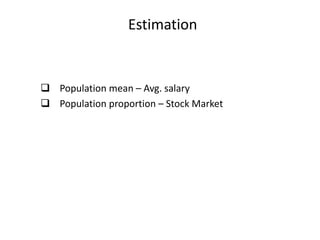
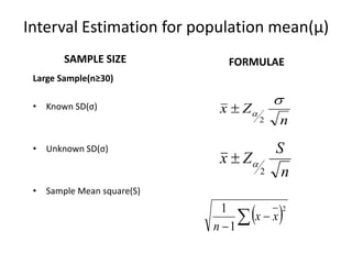
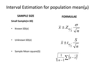
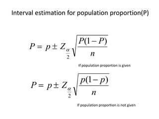
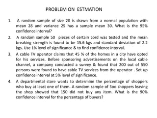
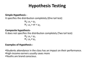
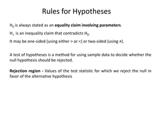
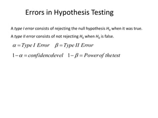
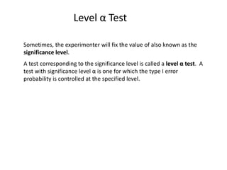
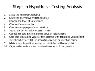
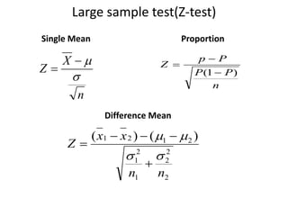
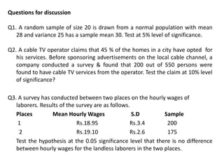
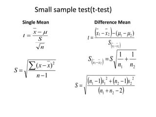
This document provides an overview of statistical inference. It discusses descriptive statistics, which summarize data, and inferential statistics, which are used to generalize from samples to populations. Key concepts covered include estimation, hypothesis testing, parameters, statistics, confidence intervals, significance levels, types of errors. Examples are given of how to calculate confidence intervals for means and proportions and how to perform hypothesis tests using z-tests and t-tests. Steps for conducting hypothesis tests are outlined.

1. Statistical Inference
By
Dr. Manas Kumar Pal

3. Statistics
It is a branch of mathematics used to summarize, analyze & interpret a
group of numbers of observations.
Types of Statistics
• Descriptive Statistics :
It summarize data to make sense or meaning of a list of numeric values.
• Inferential Statistics :
It is used to infer or generalize observations made with samples to the
larger population from which they were selected. Broadly it is classified into
theory of estimation and testing of hypothesis

4. Estimation & Testing of Hypothesis
Estimation
The method to estimate the value of a population parameter from the
value of the corresponding sample statistic.
Testing of Hypothesis
A claim or belief about an unknown parameter value.

5. Types of Estimation
• Point estimation
It is the value of sample statistic that is used to estimate most likely value of
the unknown population parameter.
Methods of point estimation
Method of maximum likelihood
Method of least squares
Method of moments
• Interval estimation
It is the range of the values that is likely to have population parameter value
with a specified level of confidence.

6. Properties of estimation
• Consistency
The statistic tend to become closer to population parameter as the sample
size increases.
• Unbiasedness
E(Statistic) = Parameter
• Efficiency
Refers to the size of the standard error(SE).
E.g., SE of sample median is greater than the sample mean, So the sample
mean is more efficient .
• Sufficiency
Refers to the usage of sample information by the statistic. E.g., Sample
mean is more sufficient than sample median because usage is more.

7. Drawback of point estimation
No information is available regarding its reliability i.e., how close it is to
its true population parameter.
In fact, the probability that a single sample statistic actually equals to the
population parameter is extremely small

8. Interval Estimation
Confidence Interval= Point estimate ± margin of error
Margin of error
= (critical value of ‘Z’ or ‘t’ at 90%, 95% & so on confidence level) x
(standard error of particular statistic)

9. Estimation
 Population mean – Avg. salary
 Population proportion – Stock Market

10. Interval Estimation for population mean(µ)
SAMPLE SIZE
Large Sample(n≥30)
• Known SD(σ)
• Unknown SD(σ)
• Sample Mean square(S)
FORMULAE
n
S
Zx
2

n
Zx


2

 2
1
1
 

xx
n

11. Interval Estimation for population mean(µ)
SAMPLE SIZE
Small Sample(n<30)
• Known SD(σ)
• Unknown SD(σ)
• Sample Mean square(S)
FORMULAE
n
S
tx
2

n
Zx


2

 2
1
1
 

xx
n

12. Interval estimation for population proportion(P)
n
PP
ZpP
)1(
2

 
n
pp
ZpP
)1(
2

 
If population proportion is given
If population proportion is not given

13. 1. A random sample of size 20 is drawn from a normal population with
mean 28 and variance 25 has a sample mean 30. What is the 95%
confidence interval?
2. A random sample 50 pieces of certain cord was tested and the mean
breaking strength is found to be 15.6 kgs and standard deviation of 2.2
kgs. Use 1% level of significance & to find confidence interval.
3. A cable TV operator claims that 45 % of the homes in a city have opted
for his services. Before sponsoring advertisements on the local cable
channel, a company conducted a survey & found that 200 out of 550
persons were found to have cable TV services from the operator . Set up
confidence interval at 5% level of significance.
4. A departmental store wants to determine the percentage of shoppers
who buy at least one of them. A random sample of 5oo shoppers leaving
the shop showed that 150 did not buy any item. What is the 90%
confidence interval for the percentage of buyers?
PROBLEM ON ESTMATION

14. 5. A manufacturer of computer paper has a production process that operates
continuously throughout an entire production shift. The paper is expected
to have a mean length 11 inches and the standard deviation of length
known to be 0.02 inch. At periodic intervals, samples are selected to
determine whether the mean paper length is still equal to 11 inches or
something has gone wrong in the production process to change the length
of the paper produced. If such a situation has occurred, corrective action
is needed. Suppose a random sample of 100 sheets is selected. And the
mean paper length is found to be 10.998 inches. Set up 95% and 99%
confidence interval estimate of the population mean paper length.
6. An operation manager for a large newspaper wants to determine the
proportion of newspapers printed that have a nonconforming attribute,
such as excessive rub-off, improper page setup, missing pages, and
duplicate pages. The operation manager determines that a random
sample of 200 newspapers should be selected for analysis. Suppose that,
of this sample of 200, 35 contain some type of non conformance. If the
operations manager wants to have 90% confidence of estimating the true
population proportion. Set up the interval estimate.

15. Critical values of Z
Level of significance(α) 10% 5% 1%
Critical values for two-
tailed test
±1.645 ±1.96 ±2.58
Critical values for left-
tailed test
-1.28 -1.645 -2.33
Critical values for right-
tailed test
1.28 1.645 2.33

16. Test of hypothesis
Hypothesis
Statements about characteristics of populations, denoted as H.
Types of Hypothesis
 Null & Alternative hypothesis
 Simple & Composite hypothesis

17. Hypothesis Testing
Null Hypothesis-
The hypothesis actually tested is called the null hypothesis. It is denoted as H0.
It is the claim that is initially assumed to be true.
Alternative Hypothesis-
The other hypothesis, assumed true if the null is false, is the alternative
hypothesis. It is denoted as H1 or Ha . Ha may usually be considered the
researcher’s hypothesis.
These two hypotheses are mutually exclusive and exhaustive so that one is
true to the exclusion of the other.
Possible conclusions from hypothesis-testing analysis are reject H0 or fail to
reject H0.

18. Hypothesis Testing
Simple Hypothesis -
It specifies the distribution completely (One tail test)
H0: μ1 = μ2
H1: μ1 > or < μ2
Composite hypothesis-
It does not specifies the distribution completely (Two tail test)
H0: μ1 = μ2
H1: μ1 ≠ μ2
Examples of Hypothesis :
Students attendance in the class has an impact on their performance.
high-income earners usually saves more
Youths are brand conscious.

19. Rules for Hypotheses
H0 is always stated as an equality claim involving parameters.
H1 is an inequality claim that contradicts H0.
It may be one-sided (using either > or <) or two-sided (using ≠).
A test of hypotheses is a method for using sample data to decide whether the
null hypothesis should be rejected.
Rejection region - Values of the test statistic for which we reject the null in
favor of the alternative hypothesis

20. Errors in Hypothesis Testing
A type I error consists of rejecting the null hypothesis H0 when it was true.
A type II error consists of not rejecting H0 when H0 is false.
ErrorIITypeErrorIType  
testtheofPowerlevelconfidence   11

21. Level α Test
Sometimes, the experimenter will fix the value of also known as the
significance level.
A test corresponding to the significance level is called a level α test. A
test with significance level α is one for which the type I error
probability is controlled at the specified level.

22. Steps in Hypothesis-Testing Analysis
1. State the null hypothesis(H0)
2. State the alternative hypothesis (H1 )
3. Choose the level of significance
4. Choose the sample size
5. Choose the appropriate test statistic
6. Set up the critical value of test statistic
7. Collect the data & calculate the value of test statistic
8. Compare calculated value of test statistic with tabulated value of test
statistic whether it falls in acceptance region or rejection region
9. Make a decision (either accept or reject the null hypothesis)
10. Express the statistical decision in the context of the problem

23. Large sample test(Z-test)
n
X
Z



Single Mean
Difference Mean
Proportion
2
2
2
1
2
1
2121 )()(
nn
xx
Z





n
PP
Pp
Z
)1( 



24. Questions for discussion
Q1. A random sample of size 20 is drawn from a normal population with mean
28 and variance 25 has a sample mean 30. Test at 5% level of significance.
Q2. A cable TV operator claims that 45 % of the homes in a city have opted for
his services. Before sponsoring advertisements on the local cable channel, a
company conducted a survey & found that 200 out of 550 persons were
found to have cable TV services from the operator. Test the claim at 10% level
of significance?
Q3. A survey has conducted between two places on the hourly wages of
laborers. Results of the survey are as follows.
Places Mean Hourly Wages S.D Sample
1 Rs.18.95 Rs.3.4 200
2 Rs.19.10 Rs.2.6 175
Test the hypothesis at the 0.05 significance level that there is no difference
between hourly wages for the landless laborers in the two places.

25. n
S
x
t


Single Mean Difference Mean
1
)( 2




n
xx
S
 
 21
)( 2121
xx
S
xx
t




 
21
11
21
nn
SS xx

   
 2
11
21
2
22
2
11



nn
snsn
S
Small sample test(t-test)

26. Small sample test(t-test)
Test for single mean
The average breaking strength of steel rods is specified to be 18.5 thousand kg. For
this a sample of 14 rods was tested . The mean & standard deviation obtained
were 17.85 and 1.955 respectively. Test at 5% level of the significance of the
deviation.
Test for difference mean
The average life of sample of 10 electric light bulbs was found to be 1456 hours
with standard deviation of 423 hours. A second sample of 17 bulbs chosen from a
different batch showed a mean life of 1280 hours with standard deviation of 398
hours. Is there a significant difference between the means of two batches. Test at
5% level of the significance.

27. Chi-square test
• Chi-square analysis is primarily used to deal with categorical (frequency)
data
• We measure the “goodness of fit” between our observed outcome and
the expected outcome for some variable
• With two variables, we test in particular whether they are independent of
one another using the same basic approach.
2
2 ( )O E
E


 
test2


28. THANK YOU