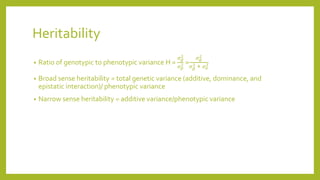
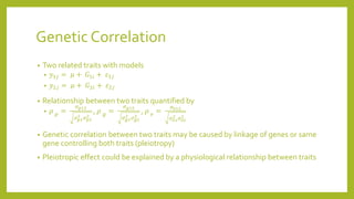
Downloaded 326 times

![Dominance Deviation (DD)
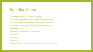
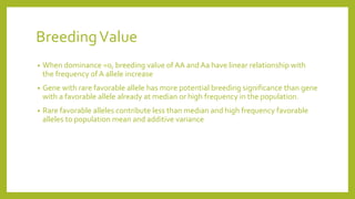
• Breeding values for a single locus are additive effects of genotypic values
• Dominance deviation is portion of genotypic values which cannot be explained by
breeding values
• Obtained by subtraction of breeding value from the genotypic value
• DD for AA: 2q(a-pd) -2p[a+ (q-p)d]=-2𝑞2
a, for Aa= 2pqd, and for aa=-2𝑝2
a](https://image.slidesharecdn.com/quantitativegenetics-160715085022/85/Quantitative-genetics-7-320.jpg)

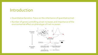
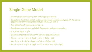
1) Quantitative genetics focuses on inheritance of quantitative traits controlled by multiple genes and influenced by the environment. 2) A basic single-gene model is used to explain quantitative genetic theory, including calculations of population mean, genetic effects, and variance components. 3) More complex multi-gene models and analyses like ANOVA and heritability are then introduced to better capture quantitative traits controlled by numerous genes and environmental influences.